Convex Optimization
Convex optimization is of two types:
- Unconstrained
- Constrained (Equality & Inequality).
Let’s learn a few convex optimization techniques from the below list.
Unconstrained Optimization
- Gradient Descent
- Newton’s Method
Equality Constrained
- Lagrangian Method
- Newton’s Method
Inequality Constrained
- Barrier’s Method
- Lagrangian Method
1. Unconstrained Optimization
1.1 Gradient Descent:
I encourage you to refer to “Gradient Descent” by Jinchuan He on blog’s page.
1.2 Newton’s Method :
Newton’s method, as outlined below, is sometimes called the damped Newton method or guarded Newton method, If there is fixed step size t = 1 then it is pure Newton method
Given a starting point $x \in \textrm{dom} \space f, \textrm{tolerance} \space \epsilon > 0$.
Repeat the following steps:
- Compute the Newton step and decrement $∆ x,λ(x).$
- Stopping criteria. quit if $(\lambda^2) / 2 ≤ ε.$
- Line search. Choose step size t by backtracking line search.
- Update. $x := x + t∆ x.$
General forms of Newton’s Method:
- Find $x$ satisfying $ g(x) = 0$ . (Finding roots of $ g(x) = 0 $)
This form is an iterative way to solve for roots of differentiable function g(x), used mainly in calculus
- Find $x$ minimizing $f (x)$ (at min $f (x) ⇒ f ′(x) = 0$ )
This form is an iterative way to solve solutions to f ′(x) = 0 . These solutions may be minima, maxima, or saddle points. This form is more relevant to Convex Optimization
Derivation of the newton step ∆x
The $2^{nd}$ order Taylor’s Expansion is given by,
\[f (x_k + t) ≈ f (x ) + f'(x_k ) * t + \frac{1}{2} f''(x_k ) * t^2\]We can write $x_k + t$ as $x_{k+1}$ i.e., the $(k+1)^{th}$ term
We know that, for ‘t’ to be optimal, we have to solve for \(\frac{df(x_k + t)}{dt} = 0\)
\[\begin{aligned} & \textrm{Now, } \space \frac{df(x_k + t)}{dt} = 0 \\ & \Rightarrow \frac{d (f (x_k )+f'(x_k ) * t+ \frac{1}{2} f''(x_k ) * t^2)}{dt} = 0 \\ & \Rightarrow f '(x_k ) + f''(x_k) t = 0 \\ & \Rightarrow t = − \frac{f'(x_k)}{f''(x_k)} \\ % & \begin{aligned} % \textrm{Now, we substitite t in} \space x_{k+1} &= x_k + t \\ % \Rightarrow x_{k+1} &= x_k − \frac{f'(x_k)}{f''(x_k)}\\ % \end{aligned} & \textrm{Now, we substitute t in} \space x_{k+1} = x_k + t \\ & \Rightarrow x_{k+1} = x_k − \frac{f'(x_k)}{f''(x_k)}\\ \end{aligned}\]Note:
- dom($f$): domain of $f (x)$ i.e., set of all real numbers $x$ where $f (x)$ is defined.
- Backtracking line search is a way to find out the hyperparameter- learning rate “ $t$ “
Intuition: Newton’s optimization method approximates the objective function by a quadratic function around the current point. By fitting a quadratic function, we can find the minimum or maximum of the quadratic function, which is close to the true minimum or maximum of the original function.
The 1st derivative gives slope of $f (x)$, 2nd derivative/ Hessian Matrix gives curvature of $f (x)$
Comparison between Redline - Newton’s method & Greenline - Gradient Descent for minimizing a func- tion. Newton’s method reaches minimum point faster by taking the curvature of
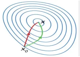
I’ll simplify this by taking the classic example of hiking a mountain to its lowest point. In gradient descent, you take the steepest descent at each step, so you miss out on the information of how the overall terrain is, let’s say obstacles, cliffs, and valleys are neglected and consume more time to navigate through all the obstacles. Now in Newton’s method you have information on the landscape of the whole terrain, which helps you avoid obstacles and reach the lowest point of the mountain much faster.
Additional Information:
- Newton’s method is very sensitive to the initial point, and can be problematic. The below image shows how big the influence of the initial point is on the convergence.
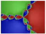 Image credits: Wikipedia
- In the upgraded Quasi-Newton approach, we can avoid calculating hessian and its inverse
- We can also solve constrained optimization problems, which broadly includes writing the Lagrange function and solving it similar to Newton’s method discussed above; I highly recommend you to read into it
2. Constrained Optimization
2.1 Lagrangian Multipliers(equality constrained) :
The basic idea is to convert the constrained optimization to an unconstrained optimization problem by multiplying the constraint with a penalty term(scalar) and adding it to the objective function.
\[\min_{\theta} \space f(\theta) \quad\textrm{s.t.} \quad g_i(\theta) = 0 \quad \forall \ i = 1...n \quad \stackrel{\text{convert}}{\Longrightarrow} \quad \min_{\vec{\theta}} \max_{\vec{\alpha}} \underbrace{L\{\overbrace{\theta_1,\alpha_1, \ldots \alpha_n}^{\text{Lagrange multipliers}}\}}_{\text{Lagrange function}} = f(\theta) + \sum_{i=1}^n \alpha_i g_i(\theta)\]Solutions:
\[\begin{aligned} & \left.\frac{\partial L}{\partial \theta}\right|_{\theta^*, \alpha} = \frac{\partial f(\theta)}{\partial \theta} + \alpha_i \frac{\partial g_i(\theta)}{\partial \theta} \Rightarrow \theta^* \\ & \left.\frac{\partial L}{\partial \alpha}\right|_{\theta, \alpha^*} \Rightarrow g_i(\theta)=0 \Rightarrow \alpha^* \quad \text{[substitute} \ \alpha^* \ \text{in first equation to get} \ \theta^*] \end{aligned}\]- Lagrange multiplier $α$ or $\lambda \in \mathbb{R}$
- An $\alpha$ exists such that partial derivative of objective function $f (x)$ at optimal point $x^∗$ is equal to product of $\alpha$ and partial derivative $g(x^∗).$
You all might know the steps of the Lagrangian method already. Now let’s dive into the intuition of the method and why it makes sense to multiply a scalar to constraint, and adding it to objective function solves our problem.
Intuition:
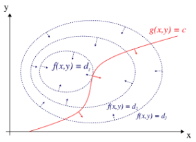
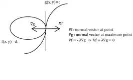
Fig: 2.4
Let’s understand this figure. Firstly, picture the graph in 3d contour plot. Our goal is to find the maximum point of f (x,y) satisfying constraint g(x,y) = c. To get there, consider contour plot of f (x,y) {contour plot is nothing but a collection of all the curves f (x,y) = d1,d2,….dn }, there exists one such curve that is tangent to the constraint function. This indicates their tangents are same for both objective function and constraint, But this also means that their normal vector to the tangents are also related. (relation can be seen in the next image, where $\lambda$ - Lagrange multiplier)
Solving this above relation simultaneously with the constraint g(x,y) = c gives us the solutions of the functions, which is the same as above derivation.
Lagrange optimization (Inequality constraints):
Similar to the equality constraints case, we modify the objective function and solve for the solutions.
\[\begin{aligned} \min_{\theta} \quad & f(\theta)\\ \textrm{s.t.} \quad & g_i(\theta)=0 \quad \forall \ i=1 \ldots n \\ & h_j(\theta) \le 0 \quad \forall \ j=1 \cdots p \end{aligned} \quad \stackrel{\text{convert}}{\Longrightarrow} \quad \min_{\vec{\theta}} \max_{\alpha, \beta} L(\theta, \alpha, \beta) = f(\theta) + \sum_{i=1}^n \alpha_i g_i(\theta) + \sum \beta_j h_j(\theta)\]Solutions:
\[\begin{aligned} & \left.\frac{\partial L}{\partial \theta}\right|_{\theta^*, \alpha, \beta} = \frac{\partial f(\theta)}{\partial \theta} + \alpha_i \frac{\partial g_i(\theta)}{\partial \theta} + \beta_j \frac{\partial h_j(\theta)}{\partial \theta} \\ & \left.\frac{\partial L}{\partial \alpha}\right|_{\theta, \alpha^*, \beta} = g_i(\theta) \Rightarrow \alpha^* \quad \text{[substitute} \ \alpha^* \ \text{and} \ \beta^* \ \text{in first equation to get} \ \theta^*] \\ & \left.\frac{\partial L}{\partial \beta}\right|_{\theta, \alpha, \beta^*} = h_j(\theta) \Rightarrow \beta^* \quad \end{aligned}\]Now we have to check if our solutions are actually the optimal solutions .
Don’t you worry KKT conditions got you, If our solution satisfies all the conditions then we can be sure it is optimal.
K.K.T (karush-kuhn-Tucker) conditions.
- $\frac{\partial L}{\partial \theta}\bigg|_{\theta, \alpha, \beta} = 0$ [Stationarity condition]
- $\frac{\partial L}{\partial \alpha}\bigg|_{θ,α,β} = 0$ [Primal feasibility]
- $\frac{∂L}{∂β}\bigg|_{θ,α,β} ≤ 0 $ [Primal feasibility]
- $β_j ≥ 0$ [Dual feasibility]
- $\sumα_ig_i(θ) = 0\ , \ \sumβ_j h_j (θ) = 0 \ \ $[Complementany slackness]
I’ll help you understand these conditions with a simple example; Consider a production company that aims to maximize its profit by deciding how many units of two products, X and Y, to produce. The company faces a budget constraint and a resource constraint, along to maximize profit.
- Stationarity : Implies that the rate at which profit increases with respect to changes in the production quantities should be balanced with the sensitivity of the constraints (budget and resource) to changes in production quantities
- Primal Feasibility : Means that the production quantities of products X and Y should satisfy the budget constraint and the resource constraint.
- Dual Feasibility : It means that the dual variables corresponding to the budget constraint and the resource constraint should be non-negative.
- Complementary Slackness : If the budget constraint is fully utilized (binding), its dual variable is positive, indicating the marginal value of additional budget. If the resource constraint has some remaining capacity (slack), its dual variable is zero, indicating that it does not affect the objective function.
Barriers Method Interior Point Method(IPM):
This very vaguely can be called an extension to Lagrangian method. Our aim remains same , converting constrained to unconstrained optimization problem. Once this is done, we can apply algorithms like Gradient descent and Newton’s method to solve it.
Let’s see how it works with a simple example.
\[\begin{aligned} \textrm{Objective function:} \quad & \textrm{Maximize the area} \ f(l,w) = \textrm{length} (l) * \textrm{width} (w)\\ \textrm{Constraint:} \quad & \textrm{Perimeter i.e.,} \quad \textrm{s.t.} \quad 2*l+2*w \le 100\\ \end{aligned}\]To apply the barrier method, we introduce a penalty term that penalizes violations of the perimeter constraint. The penalty term can be defined as the negative logarithm of the difference between the actual perimeter and the allowed maximum perimeter.
Now modified objective function looks something like this:
\[\begin{aligned} \textrm{Objective function:} \quad & \textrm{Maximize} \ B(l,w) = l*w − \mu*\log(100 − (2*l + 2*w)) \newline & \mu \ \textrm{is barrier parameter }(\mu > 0) \end{aligned}\]Intuition :
\[\begin{aligned} \textrm{min} \ f(x) \quad & \textrm{s.t.} \quad g(x) \le 0 \quad \quad \overset{\text{convert}}{\implies} \quad \quad B(x) = f (x) − \mu \log(g(x))\\ & \text{As} \ g(x) \Rightarrow 0 \textrm{ (tends to zero)}, -\log(g(x)) \rightarrow \infty \textrm{ (tends to infinity)} \end{aligned}\]Ex:
$ \text{min} \ f(x) = x \quad \text{s.t.} \quad g(x): 5-x \overset{\text{convert}}{\implies} B(x) = x − \mu \log(5 − x)$
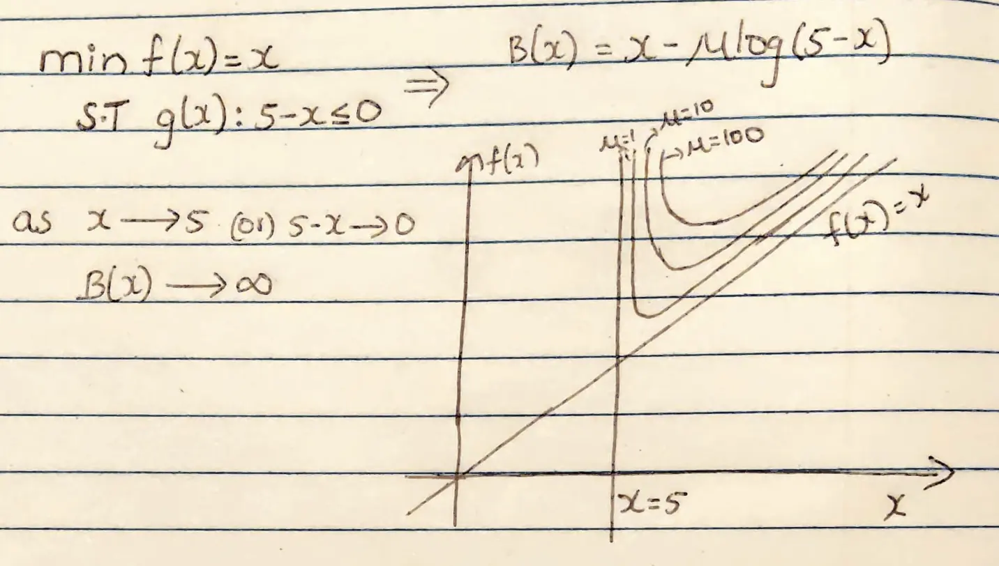
If you look at the example clearly, the barrier function $B(x)$ is not allowing the optimal x value to go beyond the constraint given. $B(x)$ is approaching infinity where x comes closer to the optimal value. It acts like a barrier stopping to cross the feasible region.
If you think about it, It’s so beautiful how a simple log function helps in solving optimization problems soo efficiently
Additional Information:
- The barrier method can be seen as a bridge between feasibility and optimality in optimization problems. By gradually reducing the barrier coefficient, it navigates the tradeoff between satisfying constraints and optimizing the objective function.
- Similar to Newton’s method, It can be sensitive to the choice of the initial point; a poor initial point, far from the feasible region, may lead to slow convergence or failure to find a feasible solution.
- Similar approach is followed if we are given equality constraints too. Hope you aren’t afraid of convex optimization anymore :)
References:
[1]Convex Optimization by Stephen Boyd
[2] Pattern Recognition and Machine Learning by Christopher Bishop
[3]Interior Point method constrained Optimization(Youtube )
[4]Constraints and Barrier Method(Youtube )
[5]Newton’s Method Linear Approximation(Youtube )
[6]Influence of Initial point(Newton’s Method)(Youtube )