Handling Imbalanced Datasets

As a young Data Scientist, you’re tasked with creating a model for a manufacturing company to predict whether a certain type of component is faulty or not. You choose your preferred classification algorithm, train it on the available data, and achieve an impressive 96.2% accuracy.

Your manager is impressed and immediately puts the model into production without further scrutiny. However, a few weeks later, your manager approaches you, frustrated that the model hasn’t identified a single faulty component since it was implemented. Upon investigation, you discover that only about 3.8% of the components produced by the company are actually defective. The model, unfortunately, has a tendency to always predict “not defective,” resulting in the high accuracy due to the imbalanced dataset.

This situation highlights the importance of addressing imbalanced class issues in classification problems, prompting us to explore various methods to tackle this challenge.

Confusion Matrix - F1 Score, Recall and Precision

An indispensable and straightforward metric for evaluating classification problems is the confusion matrix. This metric provides a comprehensive snapshot of a model’s performance, making it an excellent initial point for any classification model assessment. We encapsulate a majority of the derived metrics from the confusion matrix in the following graphical representation.

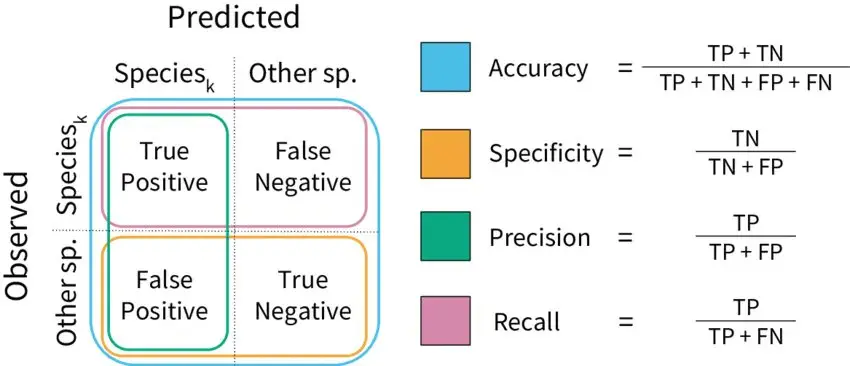
A brief overview of these metrics are as follows:

1. Accuracy: This tells us how many correct predictions our model made out of all the predictions it attempted. It’s like asking, “Out of everything it guessed, how many were right?”
2. Precision: Imagine the model saying something belongs to a certain group. Precision measures how much we can trust it when it says this. If it says something belongs to a group, how likely is it to be correct?
3. Recall: This tells us how good the model is at finding all the members of a specific group. It’s like asking, “Out of all the actual members of this group, how many did the model find?”
4. F1 Score: This is a combination of precision and recall in one metric. It helps us understand both how trustworthy the model is when it makes a claim about a group, and how well it can find all the members of that group.

Now, let’s look at different scenarios for a specific group:

• High Recall + High Precision: The model is doing an excellent job with this group. It not only finds most of them, but when it claims something belongs to this group, it’s usually right.
• Low Recall + High Precision: The model might not be great at finding all the members of this group, but when it does make a claim, it’s usually correct. So, it’s trustworthy even though it might miss some.
• High Recall + Low Precision: The model is good at finding members of this group, but it also includes some that don’t actually belong. It’s like casting a wide net, catching a lot, but also some that aren’t what we’re looking for.
• Low Recall + Low Precision: This is where the model struggles with this group. It’s not great at finding them, and when it does, it’s often wrong. This is an area where the model needs improvement.

These metrics help us understand how well our model is performing for specific groups, and whether it needs fine-tuning to be more accurate and reliable.

ROC and AUC

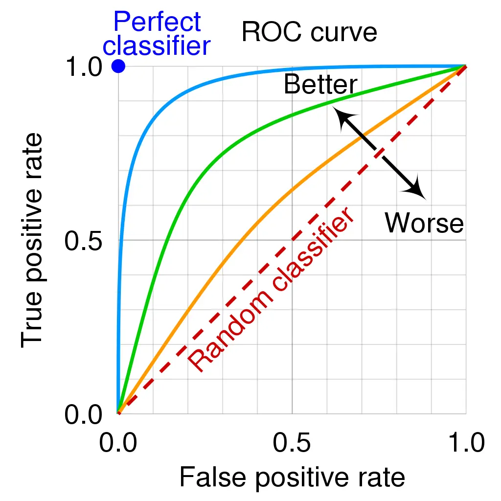
When it comes to classifying things, we need a way to measure how good our model is at distinguishing between different groups. That’s where the AUC-ROC curve comes in. Think of it like this: The curve shows us how well our model can sort things into their correct categories, based on different settings. The higher the curve, the better our model is at this job.

AUC, or Area Under the Curve, is like a score that tells us just how capable our model is at this separation task. The higher the score, the better our model is at saying “this belongs here” and “this belongs there.” To put it in a relatable example, think of a medical test. A high AUC means the test is really good at correctly identifying people with a particular condition, and those without it.The ROC curve itself is a graph. On the y-axis, we have TPR (True Positive Rate) which measures how often our model correctly identifies positives. On the x-axis, we have FPR (False Positive Rate), which tells us how often our model makes mistakes by saying something is positive when it’s not.

This curve is like a visual representation of how well our model is doing its job. The higher and farther to the left the curve is, the better our model is at distinguishing between different groups.

The Core Issue

Before we dive into solving the problem at hand, let’s take a moment to truly grasp it. We’ll do this through a straightforward example that serves two purposes: it refreshes our memory on the basics of a two-class classification, and it allows us to gain a deeper understanding of the challenge posed by imbalanced datasets. This example will serve as a foundation for the upcoming sections.

By examining this example, we’ll not only revisit the core concepts of two-class classification but also confront the crucial issue of imbalanced datasets. This scenario will serve as a reference point throughout our exploration.

A Closer Look: Imbalanced Datasets in Action

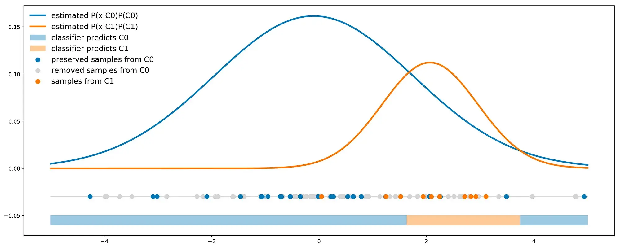
Let’s imagine a scenario where we have two distinct classes: C0 and C1. Now, here’s the interesting part: the points in class C0 are distributed along a one-dimensional Gaussian curve, centered at 0 with a variance of 4. On the other hand, points in class C1 follow a Gaussian distribution with a mean of 2 and a variance of 1. In our specific problem, a whopping 90% of our dataset belongs to class C0, leaving just 10% for class C1. This introduces a classic example of an imbalanced dataset.

To give you a visual, we’ve crafted a representative dataset of 50 points. On the right, you’ll find the theoretical distributions of both classes, perfectly reflecting their respective proportions.

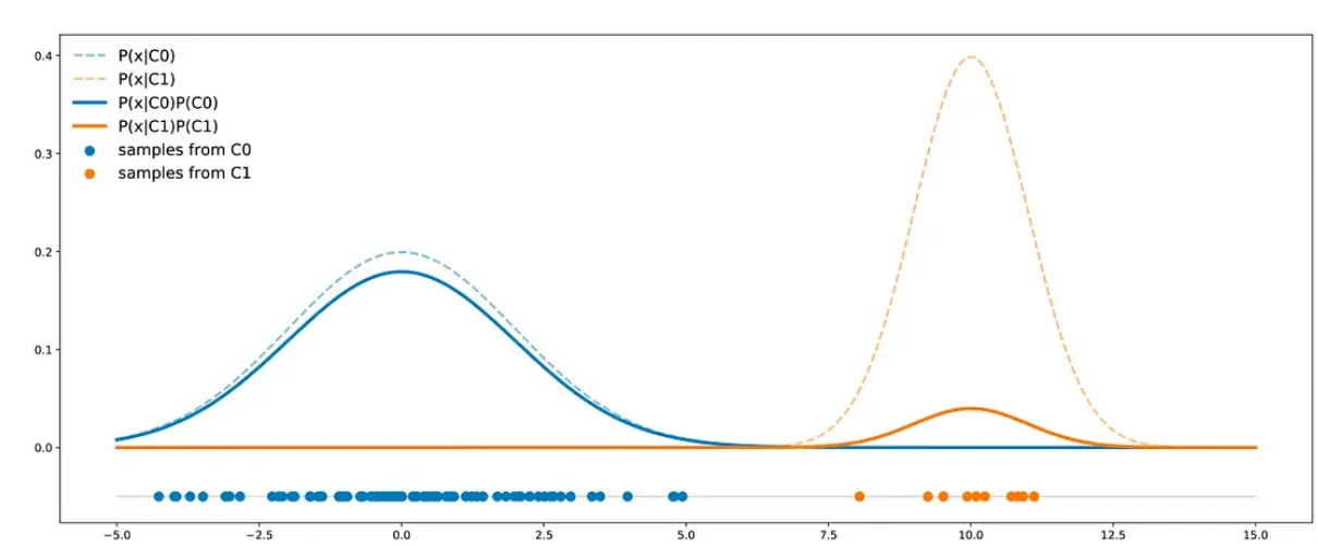
Here we see that contrarily to the previous case the C0 curve is not always above the C1 curve and, so, there are points that are more likely to be drawn from class C1 than from class C0. In this case, the two classes are separated enough to compensate the imbalance: a classifier will not necessarily answer C0 all the time.

Theoretical minimal error probability (∞)

Finally, we should keep in mind that a classifier has a theoretical minimal error probability. For a classifier of this kind (one feature, two classes), we can mention that, graphically, the theoretical minimal error probability is given by the area under the minimum of the two curves.

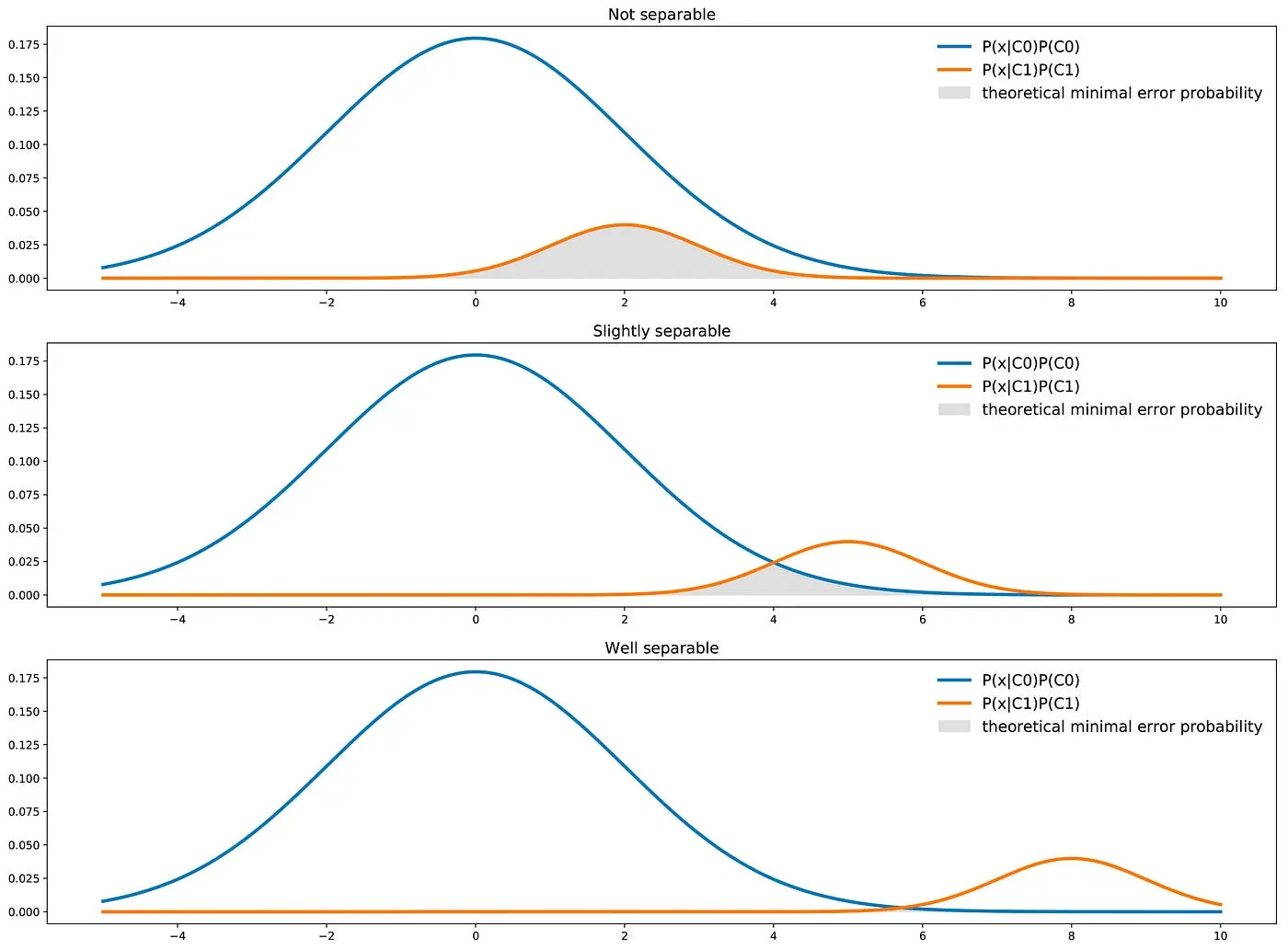
We can recover this intuition mathematically. Indeed, from a theoretical point of view, the best possible classifier will choose for each point x the most likely of the two classes. It naturally implies that for a given point x, the best theoretical error probability is given by the less likely of these two classes.

Then we can express the overall error probability as:

which is the area under the min of the two curves represented above.

Reworking the dataset and it’s pitfalls

When confronted with an imbalanced dataset, our initial instinct might be to question whether the data accurately mirrors reality. Could there be a bias in proportions due to how the data was gathered? If so, it becomes crucial to consider collecting more representative data.

Now, let’s explore what steps can be taken when the imbalance stems from the actual nature of the data. In the upcoming subsections, we’ll delve into some widely acknowledged methods for addressing imbalanced classes, focusing on adjustments made directly to the dataset itself. Specifically, we’ll navigate the potential pitfalls of undersampling, the intricacies of oversampling and synthetic data generation, and the advantages of expanding our feature set.

Undersampling, oversampling and generating synthetic data

These methods are often presented as great ways to balance the dataset before fitting a classifier on it. In a few words, these methods act on the dataset as follows:

1. Undersampling : Undersampling is a technique used to address imbalanced datasets. It involves reducing the number of instances in the overrepresented class to match the size of the underrepresented class. By doing this, the model is trained on a more balanced dataset, which can help prevent it from being biased towards the majority class. While undersampling can be effective in rebalancing the classes, it comes with a potential drawback: it discards potentially valuable information from the majority class, which could lead to loss of important insights.
2. Oversampling : Oversampling aims to mitigate this issue by increasing the representation of the minority class. Oversampling is a valuable tool for improving the performance of models on imbalanced datasets. However, it’s important to evaluate its impact on the overall model and consider potential drawbacks such as overfitting. It’s often used in conjunction with other techniques like undersampling or algorithm-level approaches for comprehensive handling of imbalanced data.
3. Generating Synthetic Data : Generating synthetic data is a technique used to address imbalanced datasets. It involves creating new, artificial data points that are similar to the existing minority class samples. This helps balance the class distribution and can improve the performance of machine learning models. There are various methods to generate synthetic data, with one of the most popular being the Synthetic Minority Over-sampling Technique (SMOTE). SMOTE works by identifying a minority class sample and creating synthetic examples along the line segments joining its nearest neighbors. This effectively increases the representation of the minority class without duplicating existing data points. Other techniques, such as ADASYN (Adaptive Synthetic Sampling), focus on generating data points in regions that are harder to learn, giving more weight to those samples.

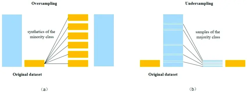
All these approaches aim at rebalancing (partially or fully) the dataset. But should we rebalance the dataset to have as much data of both classes ? Or should the majority class stay the most represented ? If so, in what proportions should we rebalance ?

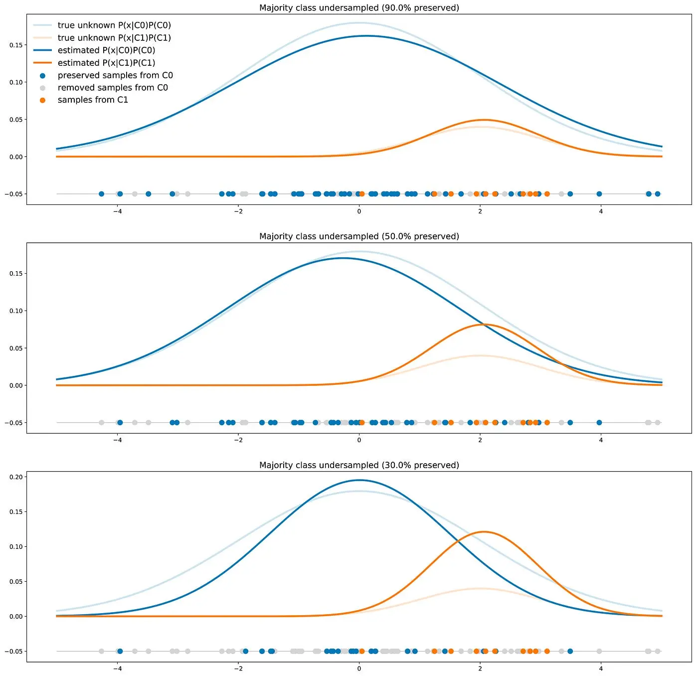
When using a resampling method (for example to get as much data from C0 than from C1), we show the wrong proportions of the two classes to the classifier during the training. The classifier learned this way will then have a lower accuracy on the future real test data than the classifier trained on the unchanged dataset. Indeed, the true proportions of classes are important to know for classifying a new point and that information has been lost when resampling the dataset.

So, if these methods have not to be completely rejected, they should be used cautiously: it can lead to a relevant approach if new proportions are chosen with purpose (we will see that in the next section), but it can also be a nonsense to just rebalance the classes without any further thoughts about the problem. To conclude this subsection, let’s say that modifying the dataset with resampling-like methods is changing the reality, so it requires to be careful and to have in mind what it means for the outputted results of our classifier.

Stratified Sampling

Stratified Sampling is a sampling method that reduces the sampling error in cases where the population can be partitioned into subgroups. We perform Stratified Sampling by dividing the population into homogeneous subgroups, called strata, and then applying Simple Random Sampling within each subgroup. As a result, the test set is representative of the population, since the percentage of each stratum is preserved. The strata should be disjointed; therefore, every element within the population must belong to one and only one stratum.

Now let’s consider a real example. The Italian population is 48.7\% males and 51.3 \% females, so a survey in Italy should be done by picking a sample of individuals while maintaining this ratio. If the survey sample contains 1000 individuals, then the Stratified Sampling picks exactly 487 males and 513 females. If Simple Random Sampling is performed, then the right percentage of males and females isn’t preserved, and the survey results will be significantly biased.

Steps Involved in Stratified Sampling

We can easily implement Stratified Sampling by following these steps:

• Set the sample size: we define the number of instances of the sample. Generally, the size of a test set is 20% of the original dataset, but it can be less if the dataset is very large.
• Partitioning the dataset into strata: in this step, the population is divided into homogeneous subgroups based on similar features. Each instance of the population must belong to one and only one stratum.
• Apply Simple Random Sampling for each stratum: random samples are taken from each stratum with the same proportion defined in the first step.

BalancedBaggingClassifier

When we try to use a usual classifier to classify an imbalanced dataset, the model favors the majority class due to its larger volume presence. A BalancedBaggingClassifier is the same as a sklearn classifier but with additional balancing. It includes an additional step to balance the training set at the time of fit for a given sampler. This classifier takes two special parameters “sampling_strategy” and “replacement”. The sampling_strategy decides the type of resampling required (e.g. ‘majority’ – resample only the majority class, ‘all’ – resample all classes, etc) and replacement decides whether it is going to be a sample with replacement or not.

Getting additional features

We discussed in the previous subsection the fact that resampling the training dataset (modifying the classes proportions) can be or not a good idea depending on the real purpose of the classifier. We saw in particular that if the two classes are imbalanced, not well separable and that we target a classifier with the best possible accuracy, then getting a classifier that always answer the same class is not necessarily a problem but just a fact: there is nothing better to do with these variables.

However, it remains possible to obtain better results in terms of accuracy by enriching the dataset with an additional feature (or more). Let’s go back to our first example where classes were not well separable: maybe can we find a new additional feature that can help distinguish between the two classes and, so, improve the classifier accuracy.

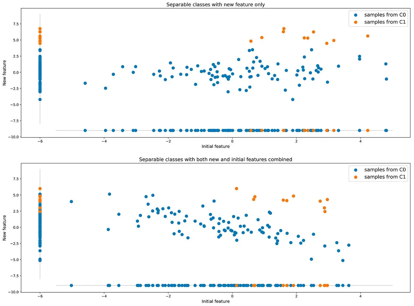
Compared to the approaches mentioned in the previous subsection that suggest to change the reality of data, this approach that consists in enriching data with more information from the reality is a far better idea when it is possible.

Restructuring the problem

Up to now the conclusion is pretty disappointing: if the dataset is representative of the true data, if we can’t get any additional feature and if we target a classifier with the best possible accuracy, then a “naive behaviour” (answering always the same class) is not necessarily a problem and should just be accepted as a fact (if the naive behaviour is not due to the limited capacity of the chosen classifier, of course).

So what if we are still unhappy with these results? In this case, it means that, in one way or another, our problem is not well stated (otherwise we should accept results as they are) and that we should rework it in order to get more satisfying results.

Cost-based classification

The feeling that obtained results are not good can come from the fact that the objective function was not well defined. Up to now, we have assumed that we target a classifier with high accuracy, assuming at the same time that both kinds of errors (“false positive” and “false negative”) have the same cost. In our example it means we assumed that predicting C0 when true label is C1 is as bad as predicting C1 when true label is C0. Errors are then symmetric.

Let’s consider our introductory example with defective (C1) and not defective (C0) products. In this case, we can imagine that not detecting a defective product will cost more to the company (customer service costs, possible juridical costs if dangerous defects, …) than wrongly labelling a not defective product as defective (production cost lost). Now, predicting C0 when true label is C1 is far worse than predicting C1 when true label is C0. Errors are no longer symmetric.

Consider then more particularly that we have the following costs:

• predicting C0 when true label is C1 costs P01
• predicting C1 when true label is C0 costs P10 (with 0 < P10 « P01) Then, we can redefine our objective function: we don’t target the best accuracy anymore but we look for the lower prediction cost instead.

Theoretical minimal cost (∞)

From a theoretical point of view, we don’t want to minimise the error probability defined above but the expected prediction cost given by :

where C(.) defines the classifier function. So, if we want to minimise the expected prediction cost, the theoretical best classifier C(.) minimises

or equivalently, dividing by the density of x, C(.) minimises

So, with this objective function, the best classifier from a theoretical point of view will then be such that:

Notice that we recover the expression of the “classic” classifier (focus on accuracy) when costs are equal.

Probability threshold

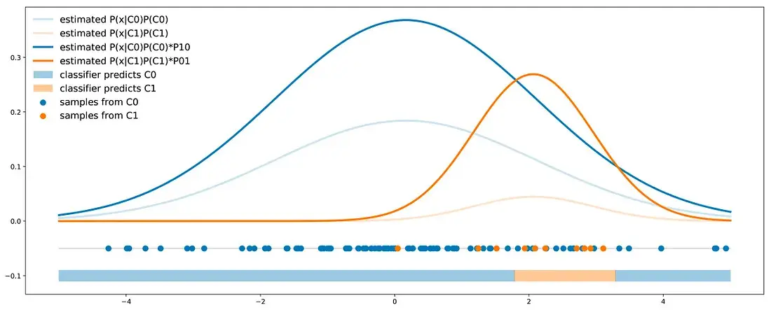
One first possible way to take into account the cost in our classifier is to do it after the training. The idea is, first, to train a classifier the basic way to output the following probabilities

without assuming any costs. Then, the predicted class will be C0 if

and C1 otherwise.

Here, it doesn’t matter which classifier we are using as long as it outputs the probability of each class for a given point. In our main example, we can fit a Bayes classifier on our data and we can then reweight the obtained probabilities to adjust the classifier with the costs errors as described.

Classes reweight

The idea of class reweight is to take into account the asymmetry of cost errors directly during the classifier training. Doing so, the outputted probabilities for each class will already embed the cost error information and could then be used to define a classification rule with a simple 0.5 threshold.

For some models (for example Neural Network classifiers), taking the cost into account during the training can consist in adjusting the objective function. We still want our classifier to output

but this time it is trained such as to minimise the following cost function

For some other models (for example Bayes classifier), resampling methods can be used to bias the classes proportions such that to enter the cost error information inside the classes proportions. If we consider the costs P01 and P10 (such that P01 > P10), we can either:

• oversample the minority class by a factor P01/P10 (cardinality of the minority class should be multiplied by P01/P10)
• undersample the majority class by a factor P10/P01 (cardinality of the majority class should be multiplied by P10/P01)

Code Samples

Random Undersampling and Oversampling

Let us first create some example imbalanced data.

from sklearn.datasets import make_classification
import pandas as pd

X, y = make_classification(
    n_classes=2, class_sep=1.5, weights=[0.9, 0.1],
    n_informative=3, n_redundant=1, flip_y=0,
    n_features=20, n_clusters_per_class=1,
    n_samples=100, random_state=10
)

X = pd.DataFrame(X)
X['target'] = y

We can now do random oversampling and undersampling using:

num_0 = len(X[X['target']==0])
num_1 = len(X[X['target']==1])
print(num_0, num_1)

# random undersample

undersampled_data = pd.concat([ X[X['target']==0].sample(num_1), X[X['target']==1] ])
print(len(undersampled_data))

# random oversample

oversampled_data = pd.concat([ X[X['target']==0], X[X['target']==1].sample(num_0, replace=True) ])
print(len(oversampled_data))

90 10
20
180

Undersampling and Oversampling using imbalanced-learn

imbalanced-learn(imblearn) is a Python Package to tackle the curse of imbalanced datasets.

It provides a variety of methods to undersample and oversample.

• Undersampling using Tomek Links: One of such methods it provides is called Tomek Links. Tomek links are pairs of examples of opposite classes in close vicinity. In this algorithm, we end up removing the majority element from the Tomek link, which provides a better decision boundary for a classifier.

from collections import Counter
from sklearn.datasets import make_classification
form imblearn.under_sampling import TomekLinks
X, y = make_classification(n_classes=2, class_sep=2,
                           weights=[0.1, 0.9], n_informative=3, n_redundant=1, flip_y=0,
                           n_features=20, n_clusters_per_class=1, n_samples=1000, random_state=20)
print('Original dataset shape %s' % Counter(y))
tl = TomekLinks()
X_res, y_res = tl.fit_resample(X, y)
print('Resampled dataset shape %s' % Counter(y_res))

Original dataset shape Counter({1: 900, 0: 100})
Resampled dataset shape Counter({1: 897, 0: 100})

Oversampling using SMOTE

In SMOTE (Synthetic Minority Oversampling Technique) we synthesize elements for the minority class, in the vicinity of already existing elements.

from imblearn.over_sampling import SMOTE

smote = SMOTE(sampling_strategy='minority')

X_sm, y_sm = smote.fit_resample(X, y)
print('Resampled dataset shape %s' % Countery_res)

Resampled dataset shape Counter({1: 897, 0: 100})

Class weights in the models

Most of the machine learning models provide a parameter called class_weights. For example, in a random forest classifier using, class_weights we can specify a higher weight for the minority class using a dictionary.

from sklearn.linear_model import LogisticRegression
clf = LogisticRegression(class_weight={0:1,1:10})

But what happens exactly in the background?

In logistic Regression, we calculate loss per example using binary cross-entropy:

In this particular form, we give equal weight to both the positive and the negative classes. When we set class_weight as class_weight = {0:1,1:20}, the classifier in the background tries to minimize:

So what happens exactly here?

If our model gives a probability of 0.3 and we misclassify a positive example, the NewLoss acquires a value of -20log(0.3) = 10.45 If our model gives a probability of 0.7 and we misclassify a negative example, the NewLoss acquires a value of -log(0.3) = 0.52 That means we penalize our model around twenty times more when it misclassifies a positive minority example in this case.

How can we compute class_weights? There is no one method to do this, and this should be constructed as a hyperparameter search problem for your particular problem.

But if you want to get class_weights using the distribution of the y variable, you can use the following nifty utility from sklearn.

from sklearn.utils.class_weight import compute_class_weight
import numpy as np

class_weights = compute_class_weight(class_weight = "balanced", classes = np.unique(y), y = y)

Key Takeaways

The Key Takeaways of the articles are as follows :

• Choose evaluation metrics for machine learning algorithms carefully to effectively assess model performance in line with your goals.
• Use resampling methods thoughtfully, avoiding them as standalone solutions and instead coupling them with a strategic reworking of the problem to achieve specific objectives.
• Reworking the problem itself is often the most effective approach for addressing imbalanced classes. This involves setting the classifier and decision rule based on a well-chosen goal, such as minimizing a cost.