Error Analysis

Error Analysis (Threshold - Cut-off selection)

Figure 1. Error Analysis

Table of contents

1. Error Analysis
   
2. Confusion Matrix
   
3. Metrics
   3.1 Accuracy
   3.2 Error
   3.3 Precision
   3.4 Recall/Sensitivity
   3.5 F1 Score
   
4. ROC Curve
   4.1 AUC (Area under the ROC Curve)
   4.2 Choosing Cutoff with Example
   

1. Error Analysis

In Classification, Error analysis is the process of examining the data points that an algorithm misclassified.

How an algorithm decides which data point belongs to which class? Using a Cut off value. Right…

A cut-off point is a certain threshold value that can be used to determine an observation belongs to which particular class. For any classification problem, the output of the model is usually a probability. The cut-off in a binary classification is the probability that the prediction is true.

Classification accuracy alone can be deceiving when dealing with imbalanced data (if there is an unequal number of observations in each class). The error rate and other metrics for any classification problem are calculated with the help of a Confusion matrix

In this post, we will learn about the Confusion matrix, its associated metrics, and Cut-off selection. We will be using Cut-off and Threshold interchangeably in this post.

2. What is the Confusion Matrix?

A Confusion matrix is an N x N matrix used to evaluate the performance of a classification algorithm, where N is the number of target classes. The matrix compares the actual target values with those predicted by the machine learning model. This gives us a holistic view of how well our classification model is performing and what kinds of errors it is making.

For a binary classification problem, we would have a 2 x 2 confusion matrix, for 3 classes, it is a 3 x 3 matrix, and so on.

Let’s take a binary classification example. The target variable for binary classification has two values, which can be Yes/No (or) True/False (or) Positive/Negative, etc. A confusion matrix uses a cut-off value and then assigns each prediction into a binary Yes/No format. It produces four different possible outcomes. Again, a cut-off (threshold) is required to build a confusion matrix.

True Positive (TP)

• The predicted value matches the actual value, where the actual value was positive and the model predicted a positive value.

True Negative (TN)

• The predicted value matches the actual value, where the actual value was negative and the model predicted a negative value.

False Positive (FP)

• The predicted value was falsely predicted, where the actual value was negative but the model predicted a positive value.
• Also known as the Type 1 error

False Negative (FN)

• The predicted value was falsely predicted, where the actual value was positive but the model predicted a negative value.
• Also known as the Type 2 error

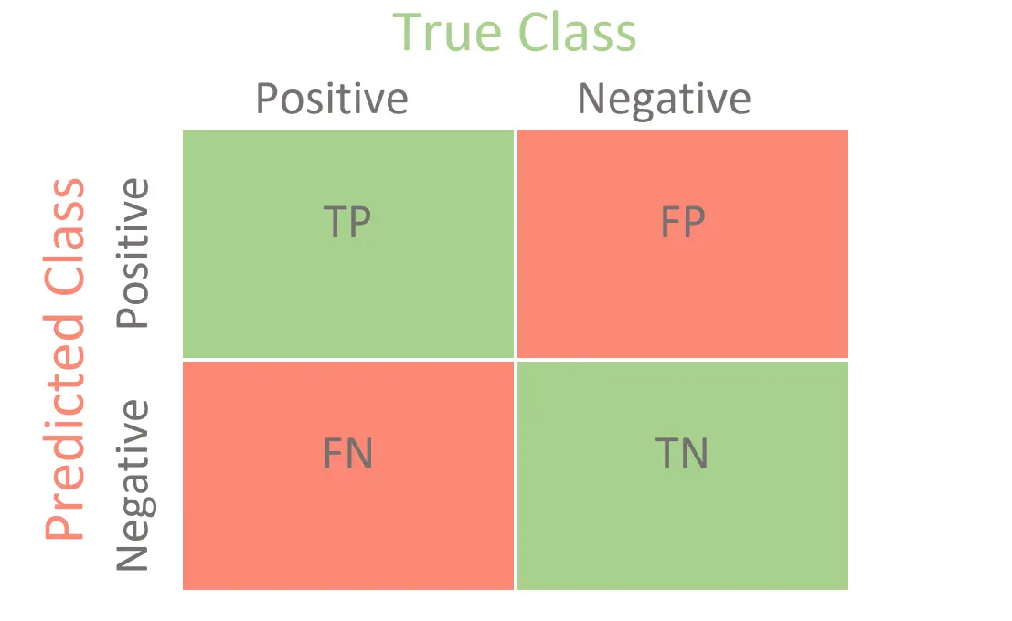
Figure 2. Confusion Matrix

What next?
For any classification problem, we need to decide which metrics are more important. Below is the list of several metrics that are often computed from a confusion matrix for a classification problem.

3. Metrics

Accuracy and Error are the most common and intuitive measures derived from a confusion matrix. We need to choose the right metric to evaluate the performance of a classification algorithm depending on the problem statement.

Let’s look at a few metrics !!

3.1 Accuracy

Accuracy is used to find how often the classifier is correct. Accuracy is the proportion of correctly classified data points among the total number of cases examined. The number of true positives and true negatives is divided by the number of true positives, true negatives, false positives, and false negatives.

Accuracy is not a reliable metric for the real performance of a classifier when there is an unequal number of observations in each class, because it will yield misleading results.

Let’s take a simple classification example of a highly imbalanced dataset. If there were 100 patients with cancer, 5 patients are diagnosed with cancer and 95 patients tested negative, the classifier could easily be biased into classifying all the samples as negative(No Cancer). It’s a terrible outcome, as 5 out of all 5 cancer patients go undiagnosed. Though the overall accuracy would be 95%, in practice the classifier would have a 100% recognition rate for the Negative class but a 0% recognition rate for the Positive class. It may obscure important differences in costs associated with different errors. In this case 1. keeping a healthy patient in the hospital (low cost), or 2. sending home a sick patient (very high cost).

3.2 Error

Error is used to find how often the classifier is incorrect. Error is the proportion of misclassified data points among the total number of cases examined. the number of false positives and false negatives divided by the number of true positives, true negatives, false positives, and false negatives.

3.3 Precision

Precision talks about how precise/accurate the model is. Precision is the measure of correctly predicted positive observations to the total predicted positive observations. Precision is also known as the Positive Predictive Value. It is a good measure to determine when the costs of False Positive are high.

When do we consider Precision as Evaluation Mesure in Classification?
Precision is a useful measure of prediction when the classes are highly imbalanced. It is more important where False Positives are more costly than False Negatives. For a good classifier, Precision should ideally be 1 (high). Precision becomes 1 only when both the numerator and denominator are equal. i.e TP = TP +FP, this also means FP should be zero. As FP increases, the value of the denominator becomes greater than the numerator, and the precision value decreases (which we don’t want). Precision is mainly used when we need to predict the positive class and there is a greater cost associated with false positives than with false negatives, such as in medical diagnosis or spam filtering.

For example, if a model is 99% accurate but only has 50% precision. It means that half of the time when it predicts a person is having cancer, it is not cancer. We mustn’t start treating a patient who doesn’t have cancer, but our model predicted it as having it (which is a False Positive).

Precision is used in conjunction with the recall to trade off false positives and false negatives. It is affected by class distribution. Precision can be thought of as a measure of exactness or quality. If we want to minimize false positives, we would choose a model with high precision. Conversely, if we want to minimize false negatives, we would choose a model with high recall.

3.4 Recall

A recall is a measure of correctly predicted positive observations over all the positive observations in the data. Recall is also known as Sensitivity (or) True Positive Rate.

When do we consider Recall as Evaluation Mesure in Classification?
The recall is more important when False Negatives are more costly than False Positive. For a good classifier, Recall should ideally be 1 (high). It becomes 1 only when the numerator and denominator are equal i.e TP = TP +FN, this also means FN should be zero. As FN increases the value of the denominator becomes greater than the numerator and the recall value decreases (which we don’t want). The recall is mainly used when we need to predict the positive class and there is a greater cost associated with false negatives than with false positives.

For example,

• We were trying to detect if an apple was poisoned or not. In this case, we would want to reduce the number of False Negatives because we do not want to classify a poisoned apple as not poisoned.
• Another example is that, for rare cancer data modeling, anything that doesn’t account for false negatives is a crime (in this case, we would want to reduce the number of False Negatives), because we do not want to classify a person as having cancer as not having cancer (therefore there is no treatment given to him/her because our model predicted so?). In this case, Recall is a better measure than precision.
• False negatives are less of a concern for YouTube recommendations. Precision is better here, i.e a video is not supposed to be recommended to a user, however, the model is recommended(not much harm/cost involved).

3.5 F1 Score

F1 Score is the weighted average of Precision and Recall. So ideally in a good classifier, we want both precision and recall to be 1, which also means False Positives(FP) and False Negatives(FN) are zero. Therefore we need a metric that takes into account both precision and recall. F1-score is a metric that takes into account both precision and recall and is defined as follows:

F1 Score becomes 1 only when precision and recall are both 1. F1 score is the harmonic mean of precision and recall and is a better measure than accuracy.

When to use F1 Score?
Using accuracy as a defining metric for a model makes sense intuitively, but more often it is always advisable to use Precision and Recall too. There might be other situations where our accuracy is very high, but our precision or recall is low. Ideally for any model, we would like to completely avoid any situations such as, where the patient has cancer, but our model classifies as him not having it i.e., aim for high recall.

Consider an example, in our dataset we can consider that achieving a high recall is more important than getting high precision, we would like to detect as many cancer patients as possible. For some other models, like classifying whether a bank customer is a loan defaulter or not, it is desirable to have a high precision since the bank wouldn’t want to lose customers who were denied a loan based on the model’s prediction that they would be defaulters.

There are also a lot of situations where both precision and recall are equally important. For example, for our model, if the doctor informs us that the patients who were incorrectly classified as suffering from cancer are equally important since they could be indicative of some other ailment, then we would aim for not only a high recall but a high precision as well. This is very easy to work with since now, instead of balancing precision and recall, we can just aim for a good F1 score and that would be indicative of a good Precision and a good Recall value as well.

4. ROC Curve

ROC curve (Receiver Operating Characteristic Curve) is a probability curve showing the performance of a classification model at all classification thresholds. It tells us how much the model is capable of distinguishing between classes. ROC shows the connection/trade-off between Sensitivity and Specificity for every possible cut-off value.

How to plot ROC Curve?
The graphical ROC curve is produced by plotting sensitivity (True Positive Rate) on the y-axis against 1–specificity (False Positive Rate) on the x-axis for the various values tabulated. A ROC curve that follows the diagonal line y=x produces false positive results at the same rate as true positive results. Therefore, we expect a diagnostic test with reasonable accuracy to have a ROC curve in the upper left triangle above the y=x line.

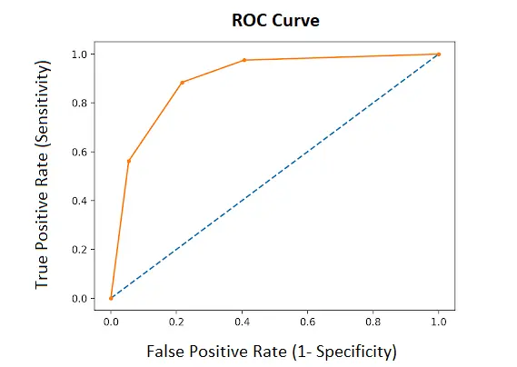
Figure 3. ROC Curve

4.1 AUC(Area under the ROC Curve)

AUC measures the entire two-dimensional area underneath the entire ROC curve, which represents the overall performance of the classification. ROC is a probability curve and AUC represents the degree or measure of separability. It tells how much the model is capable of distinguishing between classes. AUC takes values between 0 and 1, where 0 indicates a perfectly inaccurate classification and 1 reflects a perfectly accurate classification. The higher the AUC, the better the performance of the model at distinguishing between the positive and negative classes (i.e predicting 0 classes as 0 and 1 classes as 1).

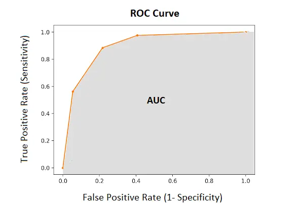
Figure 4. AUC Curve

4.2 How to choose cutoff?

The Threshold or Cut-off represents the probability that the prediction is true. The standard cutoff in any classification problem is 0.5, which means that the observation is classified as “positive” if the probability is greater than 0.5, and “Negative” otherwise. However, 0.5 is not an optimal Cut-off in all the scenarios.
Youden’s J Index, Minimizing Euclidean distance between (1-Specificity, Sensitivity) values from the point (1,1) and Profit Maximization / Cost Minimization helps in determining the optimal threshold value depending on the problem statement.

Let’s look into these methods in detail with the below example.

Example:

Let’s consider a simple example of a diagnostic test performed on the group with disease and the group without the disease. When a diagnostic test is performed, the group with the disease and the group without the disease cannot be completely divided, as overlapping may exist. the ROC curve aims to classify a patient’s disease state as either positive or negative based on test results and to find the optimal cut-off value with the best diagnostic performance. For any diagnosis, this means that even for a certain diagnostic test, the cut-off value is not universal and should be determined for each region and each disease condition.

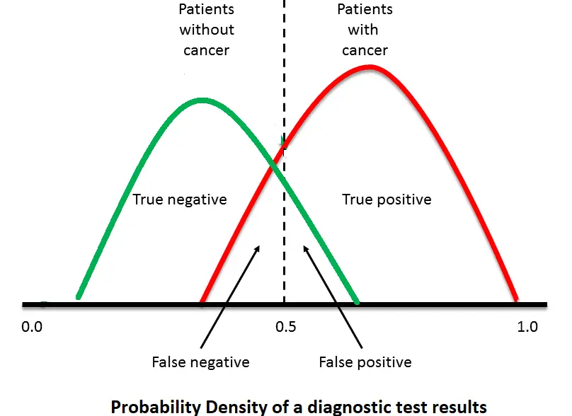
Figure 5. Overlapping datasets will always generate false positives and false negatives

• Let’s take below sample dataset with predicted probability and actual class. Predicted probability is the probability derived using our classification algorithm, and the actual class is whether a patient has cancer or not in reality.

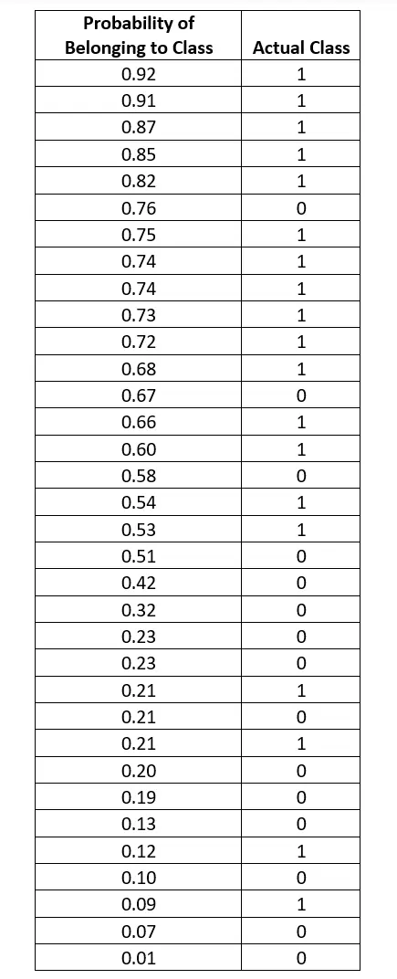
Figure 6. Sample Dataset

• Now build a confusion matrix based on threshold values 0, 0.1, 0.2, 0.3, 0.4, 0.5, 0.6, 0.7, 0.8, 0.9 and 1, derive respective True Positive Rate (Sensitivity) and False Positive Rate (1 - Specificity) to plot ROC Curve.

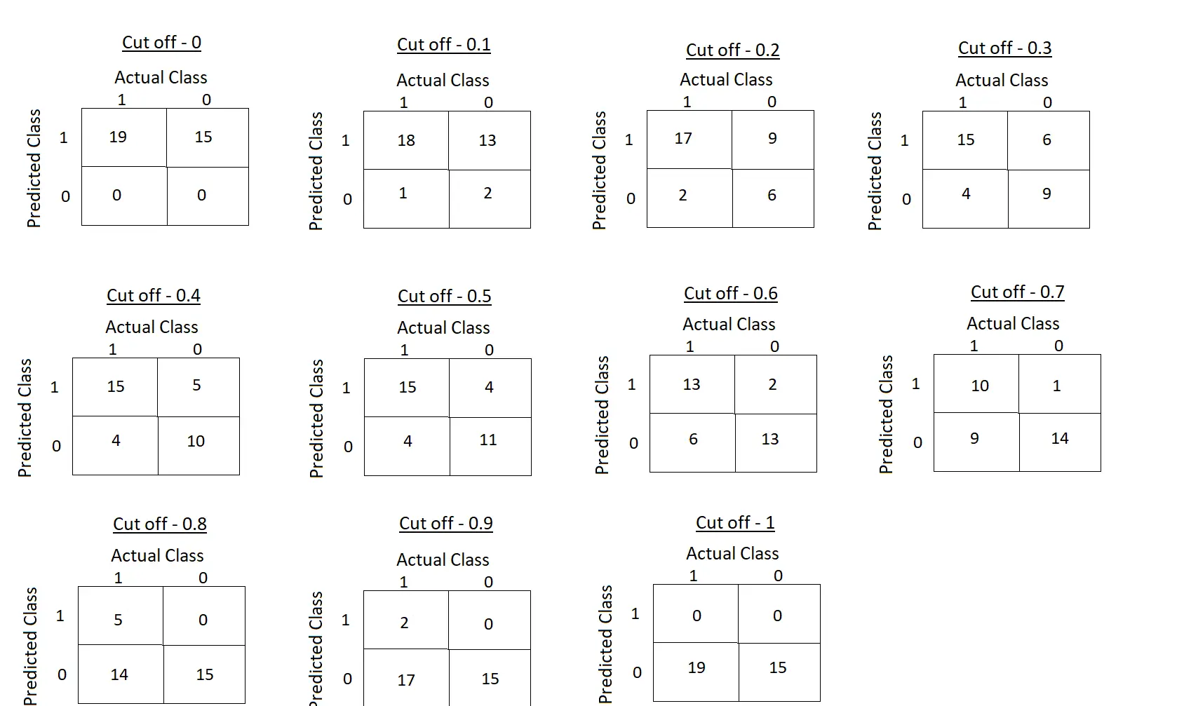
Figure 7. Confusion matrices w.r.to different cut-off selection

• Let’s derive the True Positive Rate and False Positive Rate for each cut-off value from the above sample dataset.

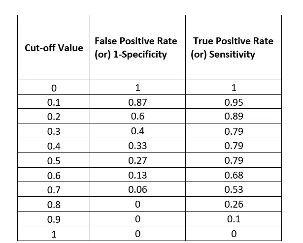
Figure 8. Sensitivity and Specificity Analysis w.r.to Cut-off

• Let’s plot the ROC Curve using the above sensitivity and 1-specificity.
  

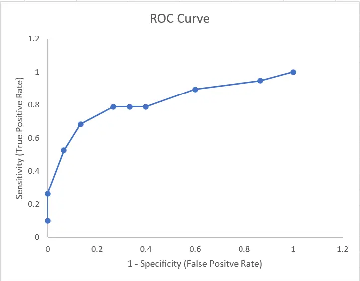
Figure 9. ROC Curve of Sample Dataset

• The cut-off value can then be selected according to the problem statement. In our case study, we would want to reduce the FALSE NEGATIVES(classifying a cancer patient as not having cancer) as much as possible, hence we need to choose a threshold value that increases the TRUE POSITIVE RATE and reduces the FALSE POSITIVE RATE.
• In our case, from the above ROC curve it is seen that, with the increase in True Positive Rate, False Positive Rate is also increasing eventually. So, we should decide the optimal cut-off depending on whether we want to detect all the positives (higher TPR) and are willing to incur some error in terms of FPR.

There are three ways to calculate the optimal cut-off :

1. Youden’s J Index.
2. Minimizing Euclidean distance between (1-Specificity, Sensitivity) from the point (1,1)
3. Profit Maximization / Cost Minimization

1. Youden’s J index

Youden’s J index is used to select the optimal cut-off. It is a diagnostic test that captures the maximum vertical distance between the ROC curve and diagonal line. The idea is to maximize the difference between True Positives and False Positives.

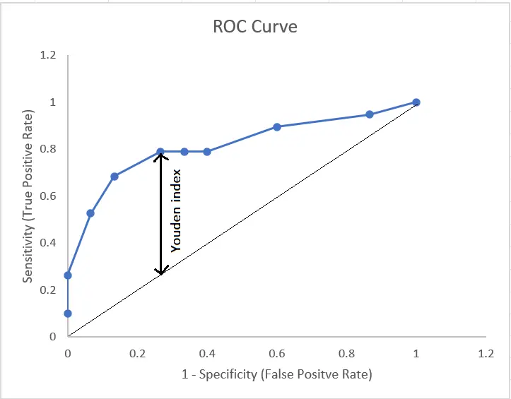
Figure 10. Cut-off selection with Youden index

2. Euclidean Distance

Another “optimal cut-off” is the value for which the point on the ROC curve has the minimum distance to the upper left corner (where sensitivity=1 and specificity=1). $$ Euclidean Distance = \sqrt{(1-sensitivity)^2 + (1-specificity)^2} $$

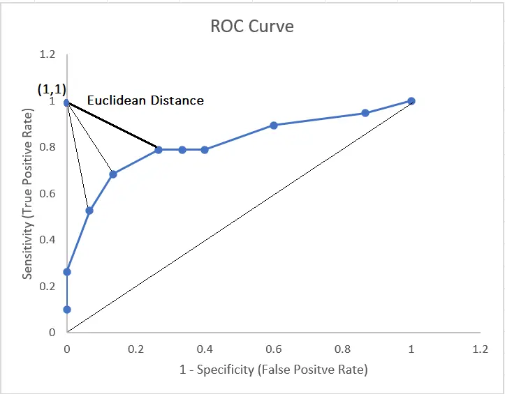
Figure 11. Cut-off selection with Euclidean Distance

3. Profit Maximization / Cost Minimization

Profit/Cost is another most useful method for determining an optimal classification probability cut-off depending on the business impact. The cost is calculated at different cutoff values to achieve a reasonable balance between false positives and false negatives. While the ROC curve helps in finding the best threshold based on the various statistics or domain expertise, a profit curve helps to pick a threshold based on the costs of true and false positive and negative predictions. It provides a sense of model sensitivity in the context of your business problem.

To summarize, in this post we have learned error analysis of a Classification problem and several ways of defining optimal ʻThresholdʼ value.