Table of contents
- Linear Regression (LR)
- LR Assumes Linear Relationship Between Features And Target
- Features Should be Independent
- Prone to Outliers
- Summary
1. Linear Regression (LR)
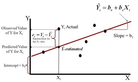
Linear regression is a simple, but efficient approach when you start to learn supervised learning with the goal of predicting the relationship between the features and target. Suppose that we have a dataset $D={(X_1, Y_1), (X_2, Y_2), \ldots, (X_n, Y_n)}$, where $x_i \in R^{1}$ for simplicity. The idea is to use an linear equation, $\hat{Y_i} = b_0 + b_1X_i$, to approximate the real target value, $Y_i$.
Moreover, $b_0, b_1$ should be calculated using the Least Square Method. In the method, we get the sum of square of differences between target and the predicted one, $J(b_0, b_1) = \sum_{i=1}^{n}(e_i)^2, e_i = Y_i - \hat{Y_i}$, then we solve $b_0, b_0$ by letting the derivative of $J$ with respect to $b_i$ equal to $0$. Instead of using this close-form solution, Gradient Descent would be another option to get those parameters.
Want more? check Math Details Behind LR. Ex 1. Figure out the strengths and weaknesses of the closed-form method and Gradient Descent, and determine under which condition you may apply what.
 Figure 1.
Linear Regression
Now, let us start to illustrate the limitations of this method.
2. Linear-Relationship between Features and Target
The biggest problem is the model can not handle non-linearity for the regression tasks. Here are two examples.
- One team explores the relationship between weight and age for students. Normally, students will grow weight along with age, then reach a plain and last a similar weight for several years, then decrease when they become old. Can linear regression display such a trend successfully? Of course not. As a consequence, finding the approximate model to suit your data is an essential part of a promising classification/regression result.
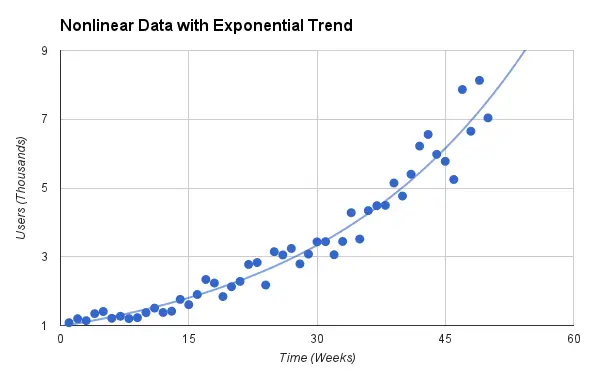
- See the exponential data in the below image, we never can find an accurate linear line to represent those points, for their non-linearity nature.
If you still want to use linear regression in the task with exponential data, \(Users = e^{a * Time}\), what can you do? Think the following steps, let $Y=log_{e}{Users}, Y = a*Time$. Now, we have a linear relationship between $Time$ and $Y$, go ahead for solving the parameter $a$. This tells us that you can apply some math transformation following your intuition or domain knowledge, letting non-linearity into linearity sometimes.
 Figure 2:
Non-linearity Between Features and Target
3. Features Should be Independent
If features are correlated, it does harm the performance of our linear model. Different metrics will mark this relationship of features for various data type. To remove the demage, We may apply some data reduction techniques to confirm the independence among features.
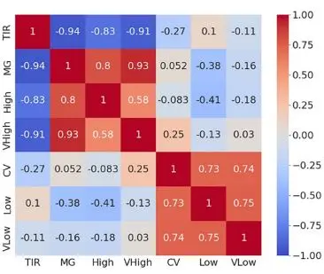
For those features with the data type of numeric, we calculate Pearson Correlation Coefficient among variables to see if it is related. For example, researchers develop a model to predict the clinician ranking based on seven standard metrics as the label of the heatmap shows. Values in the graph represent correlation coefficients. The larger/deeper the value/color is, the more related these two features are. We can clearly see that VLow is closely related to CV and Low as coefficients are 0.74 and 0.75, respectively.
For independent comparison among categorical feature, Chi-Square Test are conducted. See a hand-on example and know how to implement & visualize the Chi-Square Test.
For those higher correlated features, we may just use either of them as the input for our model building instead of all of them to remove the potential hazard on performance. You can remove them by hand or use lasso regression in an automatic way.
 Figure 3:
Correlation Between Pairs of Metrics
4. Prone to Outliers
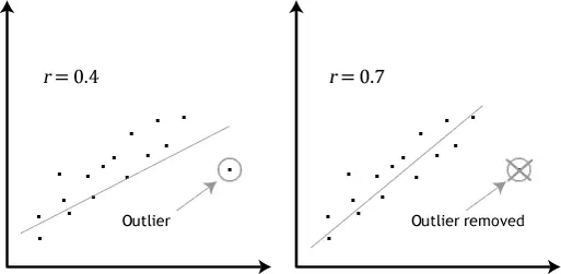
Outlier has an impact on our linear regression model. Outlier are those extreme values far away from the mean value. By removing outliers of the data points, we achieve a better approximate line for all data as the graph illustrates.
Similarly, a robust model equation integrating with the regularization will offset the damage that those outliers bring to the performance. L-1 regularization is robust against outliers as it uses the absolute value between the estimated outlier and the penalization term. Ex 2. Think why this would work? No idea about regurlarization? Find the intuitive understanding for regularization here.
To find those outliers, statistic summary, scatter plots(numeric), boxplots(categorical) can be conducted for a intuitive visualization. Then, two criterias such as Z-scores or IQR are used to detect those outliers quantitively. Finally, domain knowledge or statistical extraction will be employed for handling outliers. See section 3 in this Jupyter Notebook for detection & handle of outliers.
 Figure 4. Regression Performance Under Existing or Removed Outlier
5. Summary
In this chapter, we review linear regression for its formula, and how to solve them in two ways, close-form solution, and Gradient Descent. Then we introduce three major limitations for linear regression and point out the potential ways to avoid them whether in data processing or model robustness if you stick to this method.
Before we leave,
- Summarize the key point in each paragraph for logistics.
- Solve Ex 1-2 for those who are interested.
- Always feel free to read more online to gain a super understanding of the limitations of linear regression.