Loss functions
you are going to experience some Huh…aah!! moments in this post. let’s dive!
DISCLAIMER: I’ll try to make sense of loss functions numerically, this post doesn’t involve any mathematical proofs or equations.
Pre-School
To start with, what is an error function?
in a lame language consider preschool 4 tables… like the multiples of 4.
4 * 5 = 20 (consider 4 as a feature and 5 as a weight to be multiplied which is unknown and 20 is the target), while training a simple linear regression model, remember you initialize weights(in this case 5-still unknown) to a random number or zero. so, your linear regression model starts at ‘0’ as a weight
and train until it gets updated to 5. as follows
4 * 0 = 0 (error: 20 - 0 = 20) - error is something which the predicted value is deviated from.
4 * 1 = 4 (error: 20 - 4 = 16) - you see here error is decreased in the next step!
what did you do? - you updated the weight from 0 to 1. that is all you do in Machine Learning, you are supposed to find a weight vector/matrix/value that can lessen your error.
voila!.. now you understand that your error should decrease to get to the actual target. (small huh…ah!)
you passed pre-school
Middle School
You may ask now, okay I understand this weight concept, what is this to do anything with datasets? let’s see an example.
sample dataset
| mpg | cyl | disp | hp | drat | |
|---|---|---|---|---|---|
| MazdaRX4 | 21.0 | 6 | 160 | 110 | 3.90 |
| Mazda RX4 Wag | 21.0 | 6 | 160 | 110 | 3.90 |
| Datsun | 22.8 | 4 | 108 | 93 | 3.85 |
| Hornet 4 Drive | 21.4 | 6 | 258 | 110 | 3.08 |
| Hornet Sportabout | 18.7 | 8 | 360 | 175 | 3.15 |
unlike we have seen in pre-school, we have 5 features instead of one(4 in the preschool example).that is mpg ,cyl, disp, hp, drat.
so, as you expected we need to find 5 different weights to get the target output. let’s have a notation for weights as ‘θ’.
so our weights look like θ1, θ2, θ3, θ4, θ5.
our LR eq look like mpg * θ1 + cyl * θ2 + disp * θ3 + hp * θ4 + drat * θ5. and that’s it, you need to constantly update the weights until you hit the target.
Also, one more thing, there are 5 samples in the above dataset, so you need to sum up all 5 errors to get the total error of the model. your new objective now is to reduce total error(i.e error from all the samples).
You have pretty much seen the basics of how machine learning works numerically. Let’s see the actual content of this post.
THE COST/LOSS FUNCTION!!!
High-School
There are many different types of cost/loss functions you see on the internet, you may ask me the question, Sid, we have seen in pre-school the difference itself makes sense to calculate the loss, why do we have many kinds of them? Let’s break them down.
Regression
- MAE (mean absolute error)
- RMSE (mean squared error)
- Mean Squared Logarithmic Error Loss
- Huber Loss
Classification
- Binary Cross Entropy Loss
- Hinge Loss
- Multi-Class Cross Entropy Loss(Categorical Cross Entropy Loss)
- Kullback Leibler Divergence Loss
Regression
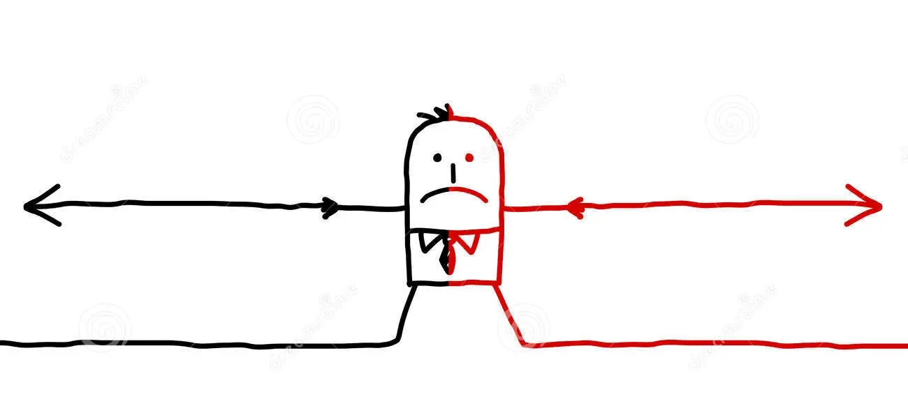
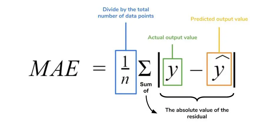
MAE: we have seen all the positivity in your algorithm, now it’s time to have some negativity! As you know Absolute value refers to making negative values positive. i.e negative error to positive in our case. from basic linear algebra, we know that the -ve sign refers to the opposite direction.
Image credits: Stock illustration
That’s how it feels if you have the same value with different signs, yes, they both cancel out and result in the wrong total error, hence we make an Absolute decision to Absolute the negative values.
Image credits: Medium
I would also like to give you an example of how to interpret MAE, in the example you have seen in middle school, say you are predicting car prices, and you got MAE of 1500, which means your model is giving +/- $1500 in error. which is +1500 is bad for the customer and -1500 is bad for the company/website.
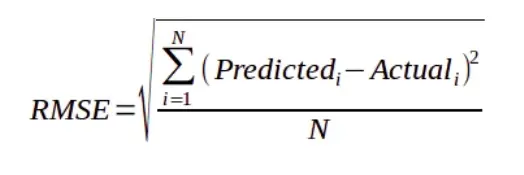
- RMSE: Let’s say some of your samples have a high error when compared to others, when taking a mean of them, you kind of neutralize the error on total error, but you missed the samples that have a high error, to handle this you kind to impose a penalty to the high error by squaring them. The squaring means that larger mistakes result in high errors than smaller mistakes, meaning that the model is punished for making larger mistakes. Doesn’t it make sense? (another small huh..ah! moment). This also handles the opposite direction vectors problem, ain’t it?
Image credits: Geeks for geeks
and of course, root mean squared error makes the value on the same scale.
- Root Mean Squared Log Error: First ill introduce the equation:
Image credits: Medium
That’s a lot in an equation compared to what we have seen earlier. let’s break it down.
+1 makes log(0) not actual being undefined or an error. where log(1) = 0.
In the case of RMSE, the presence of outliers can explode the error term to a very high value. But, in the case of RMLSE, the outliers are drastically scaled-down therefore, nullifying their effect. Let’s understand this with a small example:
| X | Y | |
|---|---|---|
| Case 1: | 30 | 35 |
| 70 | 90 | |
| 90 | 90 | |
| RMSE | 4.123 | |
| RMSLE | 0.0019 |
| X | Y | |
|---|---|---|
| Case 2: | 30 | 35 |
| 70 | 90 | |
| 90 | 90 | |
| 102 | 750 | |
| RMSE | 168.4 | |
| RMSLE | 0.7504 |
We can see that the value of the RMSE explodes in magnitude as soon as it encounters an outlier. In contrast, even on the introduction of the outlier, the RMSLE error is not affected much. From this small example, we can infer that RMSLE is very robust when outliers.
If you observe the equation. it can be re-written as log( (predicted+1) / (actual+1)), which is broadly written as relative Error error between the predicted and the actual.
let’s see a couple of examples to understand this effect:
| Y | X | RMLSE | RMSE | |
|---|---|---|---|---|
| Case 1: | 100 | 90 | 0.1053 | 10 |
| Y | X | RMLSE | RMSE | |
|---|---|---|---|---|
| Case 2: | 10000 | 9000 | 0.1053 | 1000 |
Now you should have understood the relative error that we mentioned above, RMSLE metric only considers the relative error between the Predicted and the actual value, and the scale of the error is not omitted. RMSE value Increases in magnitude as the scale of error increases.
In simple words, more penalty is incurred when the predicted Value is less than the Actual Value. and, Less penalty is incurred when the predicted value is more than the actual value.
I’ll give you a perfect example of how this works in real-world scenarios.
Consider a ride scenario like uber/lyft. you are predicting the time taken to end the ride.
if the algorithm overestimates the ride time, it’s perfectly fine to end the ride before the estimated time and acceptable.
on the contrary, if the algorithm predicts ride time is less than what it takes, the uber driver/uber gets bad reviews, which is not acceptable.
huh…ah! moment isn’t it?
- Huber Loss:
when you use the MAE in optimizations that use gradient descent, you’ll face the fact that the gradients are continuously large. This is bad for learning - it’s easy to overshoot the minimum continuously, which makes it hard to converge at the minimum. Consider Huber loss. Hold on let’s make sense of what we have just read!
Image credits: Medium
Interpreting the equation:
- In the first part, we perform this only when the absolute error is less than or equal to 𝛿 which we can configure.
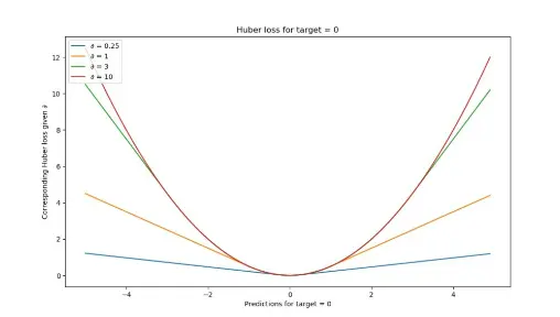
- We use the second part otherwise. let’s see how 𝛿 differs when predicting the target and respective huber loss.
Image credits: Medium
For relatively small 𝛿’s (in our case, with 𝛿 = 0.25, you’ll see that the loss function becomes relatively flat. It takes quite a long time before loss increases, even when predictions are getting larger and larger.
For larger 𝛿’s, the slope of the function increases. As you can see, the larger the 𝛿, the slower the increase of this slope: eventually, for really large 𝛿 the slope of the loss tends to converge to some maximum.
If you look closely, you’ll notice the following:
With large 𝛿, the loss becomes increasingly sensitive to larger errors and outliers. That might be good if your errors are small, but you’ll face trouble when your dataset contains outliers.
Huber loss approaches MAE when 𝛿 ~ 0 and MSE when 𝛿 ~ ∞ (large numbers.)
That means You are controlling the ‘degree’ of MAE vs MSE-ness you’ll introduce in your loss function. As we have this benefit, you may ask then why don’t we use huber every time. As you have to configure them manually you’ll have to spend time and resources on finding the most optimum 𝛿 for your dataset. This is an iterative problem that, in the extreme case, may become impractical at best and costly at worst. However, in most cases, it’s best just to experiment - perhaps, you’ll find better results!
Everything is great with regression, what if the problem is classification? which loss do we use frequently? well that’s a story for another WHAT IF
Almost forgot you passed High School.
-Siddhartha Putti
putti.s@northeasten.edu


