Learn Statistics and think Probabilities
The real-world data is often noisy with some true underlying signal. By applying Machine Learning, we hope to identify the signal from the noise. We require a language for quantifying “noise” or uncertainty. Quantification of uncertainty is the realm of Probability Theory.
Table of contents
- Probability
1.1 Basic Terminology
1.2 Marginal Probability
1.3 Joint Probability
1.4 Conditional Probability
1.5 Bayes Rule/Theorem
1.6 References - Statistics
2.1 Population
2.2 Sample
2.3 Mean
2.4 Variance
2.5 Standard Deviation
2.6 Normal/Gaussian Distribution
1. Probability
Probability is the branch of mathematics that concerns the study of uncertainty i.e, how likely an event is to occur. In simple terms, the probability is a number that reflects the chance or likelihood that a particular event will occur.
- Probabilities can be expressed as proportions that range from 0 to 1, and they can also be expressed as percentages ranging from 0% to 100%.
- A probability of 0 indicates that there is no chance that a particular event will occur, whereas a probability of 1 indicates that an event is certain to occur.
- A probability of 0.45 (45%) indicates that there are 45 chances out of 100 of the event occurring.
1.1 Basic Terminology
1. Sample Space
The set of all possible outcomes or results of an experiment is called Sample Space.
- It is commonly denoted by the labels $S$ or $\Omega$.
2. Event
A subset of the sample space is an Event. If the outcome of an experiment is included in this subset, then the event has occurred.
- It is denoted by $E$
- The Probability of event E is denoted as $P(E)$.
Example-1:
- Experiment: Tossing a single coin
- Sample space: ${H,T}$
- $H$ means that the coin was heads
- $T$ means that the coin was tails
- Possible Events:
- $E={H}$
- $E={T}$
- Probability of Events:
- $P(E=H) = \frac{1}{2}$
- $P(E=T) = \frac{1}{2}$
1.2 Marginal Probability
Marginal Probability is the probability of occurrence of a single event.
- It may be thought of as an unconditional probability. It is not conditioned on another event.
- The marginal probability of an event A is denoted as $P(A)$.
- E.g:
- The probability that a card drawn is red i.e, $P(red) = 0.5$
- The probability that a card drawn is a 4 i/e, $P(four) = 1/13$
1.3 Joint Probability
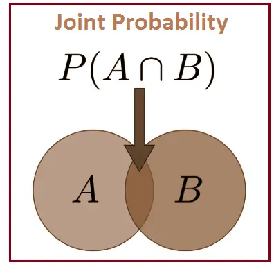
Joint probability is the probability that two events will occur simultaneously.
- The joint probability of two events A and B is denoted as $P(A,B)$ or $P(A \cap B)$.
1.4 Conditional Probability
Conditional probability is a measure of the probability of an event occurring, given that another event (by assumption, presumption, assertion, or evidence) has already occurred.
- If the event of interest is A and the event B is known or assumed to have occurred, “the conditional probability of A given B”, or “the probability of A under the condition B”, is usually written as $P(A|B)$ or occasionally $P_B(A)$.
- This can also be understood as the fraction of probability B that intersects with A.
- It is important to note that $P(A|B)$ is not the same as $P(B|A)$.
1.5 Bayes Rule/Theorem
Bayes Rule/Theorem tells us how to calculate conditional probability with the information we already have. It is a mathematical rule that describes how to update a belief, given some evidence. In other words – it describes the act of learning.
- Equation:
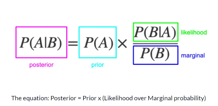
There are four parts:
- Posterior probability (updated probability after the evidence is considered)
- Prior probability (the probability before the evidence is considered)
- Likelihood (probability of the evidence, given the belief is true)
- Marginal probability (probability of the evidence, under any circumstance)

1.6 References
- Probability basics
- Bayes Rule - for beignners
- Bayes Theorem - Clearly Explained
- Bayes theorem, the geometry of changing beliefs
2. Statistics
While Probability deals with quantifying uncertainty and predicting the likelihood of future events, Statistics involves the analysis of the frequency of past events.
It concerns the collection, organization, displaying, analysis, interpretation, and presentation of data. In statistics, we apply probability(probability theory) to draw conclusions from data.
2.1 Population
A Population is a representative sample of a larger group of people (or even things) with one or more characteristics in common.
- It is denoted by $N$
2.2 Sample
A Sample is the selection of a subset of individuals from within a
statistical population to estimate the characteristics of the whole population.
- It is denoted by $n$
2.3 Mean
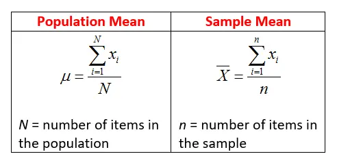
The Mean summarizes an entire dataset with a single number representing the data’s center point or typical value. It is also known as the arithmetic average, and it is one of several measures of central tendency.
- Population mean is denoted by $\mu$ while sample mean is denoted by $\bar{X}$
2.4 Variance
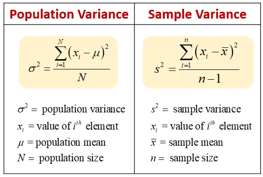
Variance is a measure of variability. It is calculated by taking the average of squared deviations from the mean. Variance tells you the degree of spread in your data set. The more spread the data, the larger the variance is in relation to the mean.
- Population variance is denoted by $ \sigma^2$ while sample variance is denoted by $s^2$
2.5 Standard Deviation
The Standard Deviation is a statistic that measures the dispersion of a dataset relative to its mean and is calculated as the square root of the variance.
- Population standard deviation is denoted by $\sigma$ while sample standard
- deviation is denoted by $s$.
2.6 Normal/Gaussian Distribution
A Normal Distribution is a continuous probability distribution of data points that appears as a bell curve when graphed using a line graph or histogram. It also goes by the name Gauss distribution, Gaussian distribution, and Laplace-Gauss distribution.
It is a parametric distribution, meaning - the information about the distribution of the population is known and is based on a fixed set of parameters, here $\mu$ and $\sigma$.
The general form of its probability density function is
\[\LARGE f(x) = \frac{1}{\sqrt{2\pi\sigma^2}}e^{-\frac{1}{2} (\frac- {x-\mu}{\sigma})^2 }\]- The parameters $\mu$ and $\sigma$ are also called location and scale parameters respectively.
Compared to other probability distributions, a normal distribution has several notable properties:
- Its graph has a distinctive symmetrical shape - A normal distribution curve appears symmetrically in the shape of a bell.
- It is characterized by equal values - The mean, median, and mode of its data set will all be the same number.
- Data distribution is equally split - Regardless of sample size and the sample mean, half the data points will be below the mean, and half the data points will be above the mean.
- It divides its data using standard deviations - A standard deviation is a measurement of how far away a data point is from the mean. The skewness of a data point will depend on the number of standard deviations it falls from the sample mean.
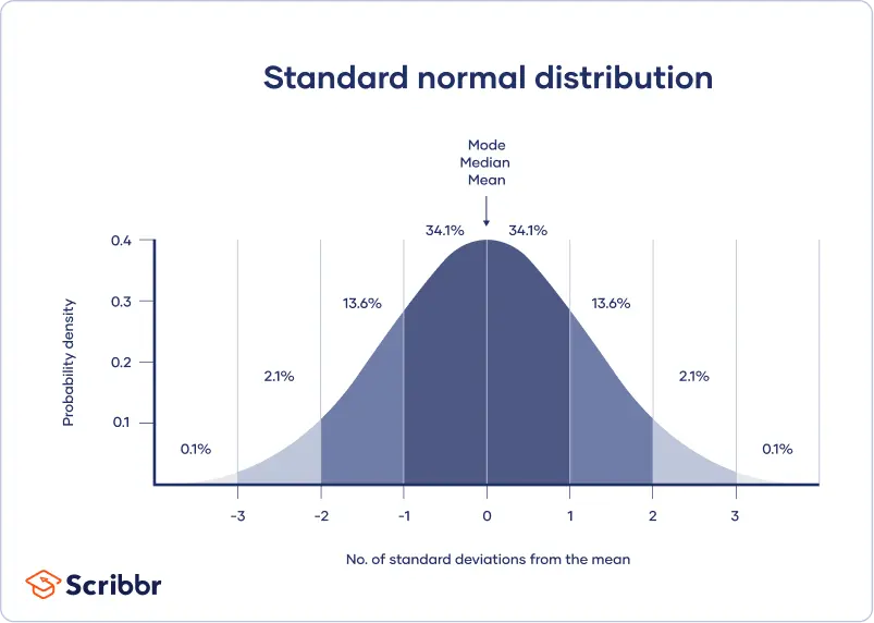
- The distribution of data follows an empirical rule of normal probability - With a normal distribution of data, 99.7 percent of all data points fall within three standard deviations from the mean in either direction. The first standard deviation of the mean covers 34.1 percent of all data points above the mean and 34.1 percent of all data points below the mean. The second standard deviation encompasses an additional 13.6 percent of data points above the mean and another 13.6 percent below the mean. The third standard deviation includes 2.1 percent of data points in either direction—both at the very top of the scale and the very bottom of the scale. This means you could fall on the ninety-ninth percentile of sample size and still be within three standard deviations of the mean. You have to be a true outlier, or special case, to go beyond three standard deviations.
- The total area under the curve has a value of one - If you were to calculate the total area under a normal distribution curve, its value would equal one unit of measure.
