Linear models are one of the simplest way to predict output using a linear function of input features.
\[\hat{y} = w[0] x[0] + w[1] x[1] + w[2] x[2] + w[3] x[3] +...+ w[n] x[n] + b\]In the equation above, we have shown the linear model based on the n number of features. Considering only a single feature as you probably already have understood that w[0] will be slope and b will represent intercept. Linear regression looks for optimizing w and b such that it minimizes the cost function. The cost function can be written as:
\[\sum_{i = 1}^{M} (y_i - \hat{y_i})^2 = \sum_{i = 1}^{M} (y_i - \sum_{j = 0}^{p} w_j x_{ij})^2\]In the equation above we have assumed the data-set has M instances and p features. Once we use linear regression on a data-set divided in to training and test set, calculating the scores on training and test set can give us a rough idea about whether the model is suffering from over-fitting or under-fitting. The chosen linear model can be just right also, if we are lucky enough! If we have very few features on a data-set and the score is poor for both training and test set then it’s a problem of under-fitting. On the other hand if we have large number of features and test score is relatively poor than the training score then it’s the problem of over-generalization or over-fitting. Ridge and Lasso regression are some of the simple techniques to reduce model complexity and prevent over-fitting which may result from simple linear regression.
Ridge Regression
In ridge regression, the cost function is altered by adding a penalty equivalent to square of the magnitude of the coefficients.
\[\sum_{i = 1}^{M} (y_i - \hat{y_i})^2 = \sum_{i = 1}^{M} (y_i - \sum_{j = 0}^{p} w_j x_{ij})^2 + \lambda \sum_{j = 0}^{p} w_j^2\]This is equivalent to saying minimizing the cost function in previous equation under the condition as below,
\[\sum_{j = 0}^{p} w_j^2 < c, for~some~c > 0\]So ridge regression puts constraint on the coefficients (w). The penalty term (lambda) regularizes the coefficients such that if the coefficients take large values the optimization function is penalized. So, ridge regression shrinks the coefficients and it helps to reduce the model complexity and multi-collinearity. Going back to the equation one can see that when λ → 0 , the cost function becomes similar to the linear regression cost function. So lower the constraint (low λ) on the features, the model will resemble linear regression model.
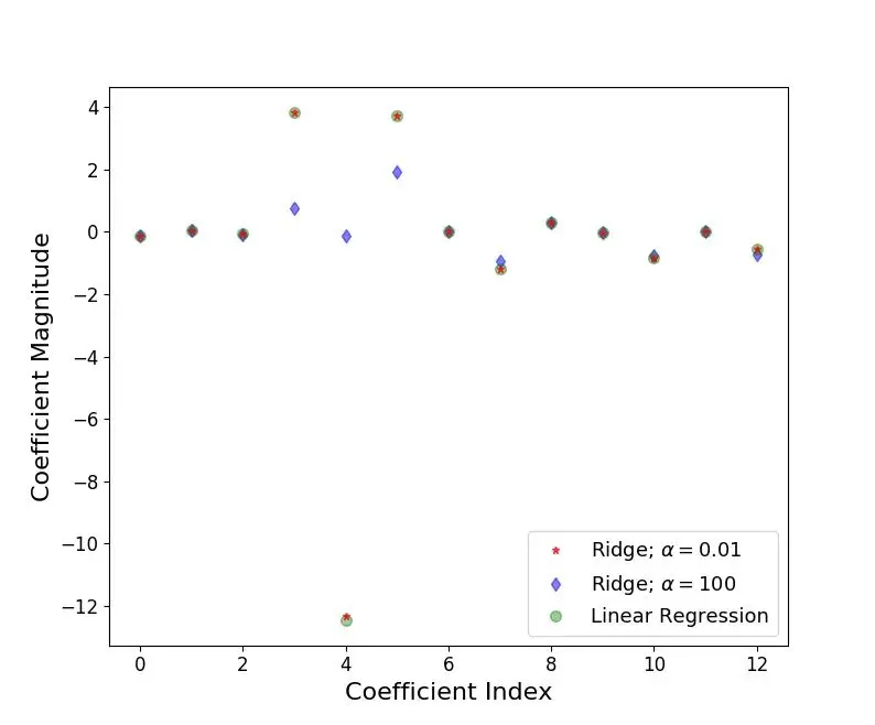
In X axis we plot the coefficient index and, for Boston data there are 13 features (for Python 0th index refers to 1st feature). For low value of α (0.01), when the coefficients are less restricted, the magnitudes of the coefficients are almost same as of linear regression. For higher value of α (100), we see that for coefficient indices 3,4,5 the magnitudes are considerably less compared to linear regression case. This is an example of shrinking coefficient magnitude using Ridge regression.
Lasso Regression
The cost function for Lasso (least absolute shrinkage and selection operator) regression can be written as,
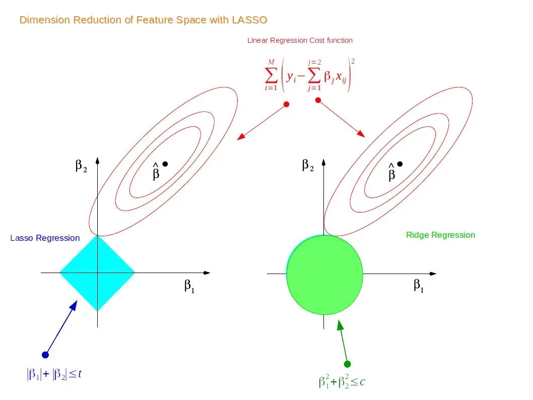
\[\sum_{i = 1}^{M} (y_i - \hat{y_i})^2 = \sum_{i = 1}^{M}(y_i - \sum_{j = 0}^{p}w_j x_{ij})^2 + \lambda\sum_{j = 0}^{p}|w_j|\] \[For~some~t > 0,~\sum_{j = 0}^{p}|w_j| < t\]Just like Ridge regression cost function, for lambda =0, the equation above reduces to linear regression equation. The only difference is instead of taking the square of the coefficients, magnitudes are taken into account. This type of regularization (L1) can lead to zero coefficients i.e. some of the features are completely neglected for the evaluation of output. So Lasso regression not only helps in reducing over-fitting but it can help us in feature selection. Just like Ridge regression the regularization parameter (lambda) can be controlled. The lasso performs shrinkage so that there are “corners’’ in the constraint, which in two dimensions corresponds to a diamond. If the sum of squares “hits’’ one of these corners, then the coefficient corresponding to the axis is shrunk to zero.
Lasso and Ridge Distribution
For a two-dimensional feature space, the constraint regions (see supplement 1 and 2) are plotted for Lasso and Ridge regression with cyan and green colours. The elliptical contours are the cost function of linear regression. Now if we have relaxed conditions on the coefficients, then the constrained regions can get bigger and eventually they will hit the centre of the ellipse. This is the case when Ridge and Lasso regression resembles linear regression results. Otherwise, both methods determine coefficients by finding the first point where the elliptical contours hit the region of constraints. The diamond (Lasso) has corners on the axes, unlike the disk, and whenever the elliptical region hits such point, one of the features completely vanishes! For higher dimensional feature space there can be many solutions on the axis with Lasso regression and thus we get only the important features selected.
Lasso tends to give sparse weights (most zeros), because the l1 regularization cares equally about driving down big weights to small weights, or driving small weights to zeros. If we have a lot of predictors (features), and you suspect that not all of them are that important, Lasso may be really good idea to start with.
Compare Ridge and Lasso :
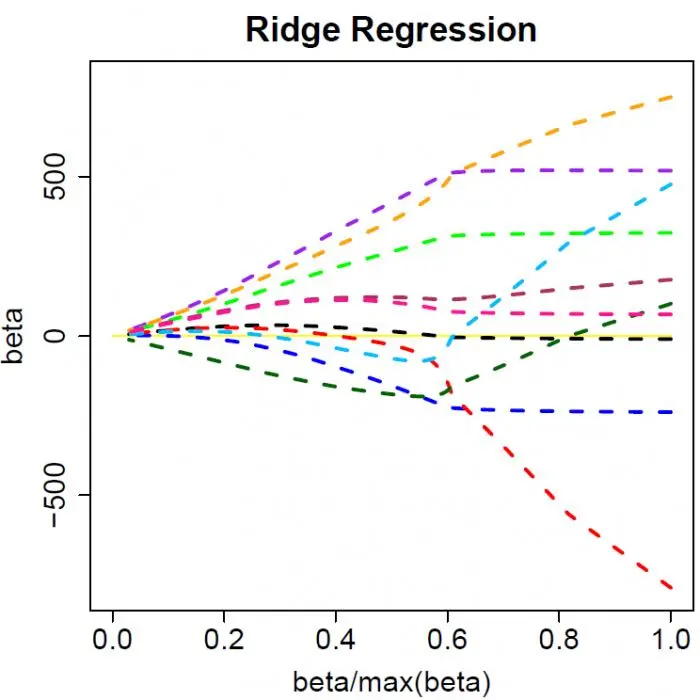
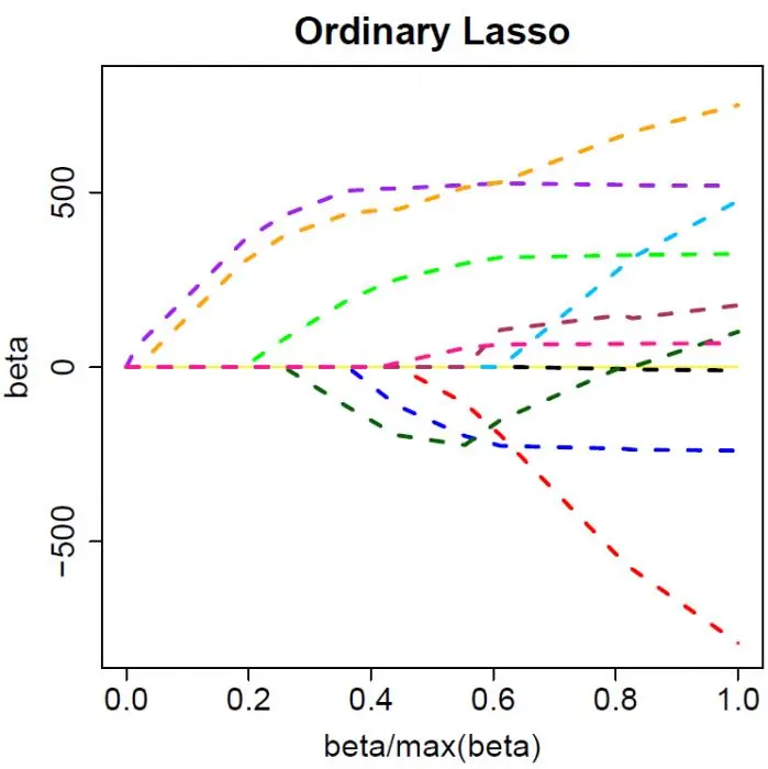
The colored lines are the paths of regression coefficients shrinking towards zero. If we draw a vertical line in the figure, it will give a set of regression coefficients corresponding to a fixed $\lambda$. (The x-axis actually shows the proportion of shrinkage instead of $\lambda$).
Ridge regression shrinks all regression coefficients towards zero; the lasso tends to give a set of zero regression coefficients and leads to a sparse solution.
Note that for both ridge regression and the lasso the regression coefficients can move from positive to negative values as they are shrunk toward zero.
 Figure 1
 Figure 2
 Figure 3
 Figure 4