Introduction
Recurrent Neural Networks (RNNs) are a type of artificial neural network that are particularly useful in modeling sequential data. They are widely used in natural language processing, speech recognition, image captioning, and many other applications. In this article, we will provide an introduction to RNNs, explaining the basic concepts and mathematical expressions involved.
Background
Before diving into RNNs, let’s review some basics of neural networks. A neural network consists of layers of interconnected nodes, or neurons, that are organized into an input layer, one or more hidden layers, and an output layer. Each neuron takes in one or more inputs, computes a weighted sum of those inputs, and applies a non-linear activation function to the result.
The weights and biases of the neurons are learned through a process called backpropagation, in which the network is trained on a set of labeled examples to minimize the error between the predicted output and the true output. This process involves iteratively adjusting the weights and biases of the neurons to improve the network’s performance.
RNNs
RNNs are a type of neural network that are designed to handle sequential data, such as time series or natural language sentences. Unlike traditional feedforward neural networks, which process all the inputs at once and produce a single output, RNNs process the inputs one at a time, and maintain an internal state that depends on the previous inputs.
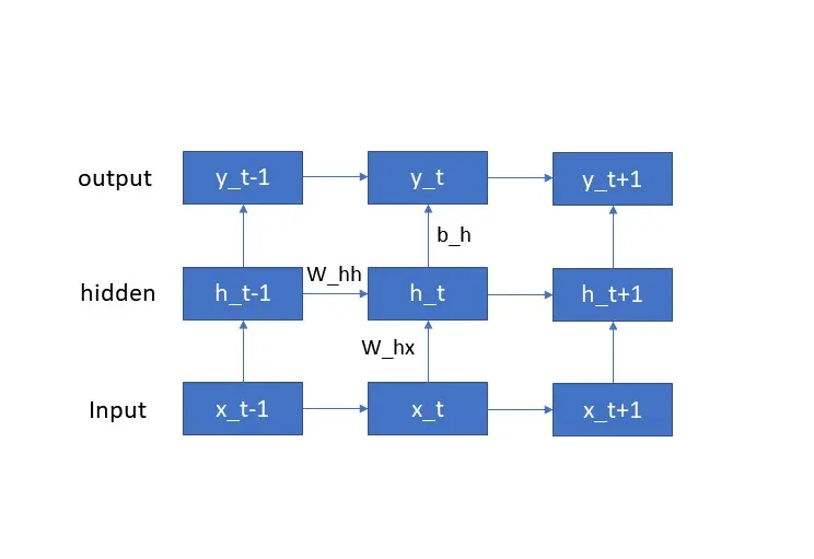
The basic structure of an RNN is shown in the below figure. At each time step, the network takes in an input $x_t$ and produces an output $y_t$, as well as updating its internal state $h_t$. The internal state is passed from one time step to the next, allowing the network to “remember” previous inputs and incorporate them into its output.

The Recurrence Formula
The internal state $h_t$ of an RNN is computed using a recurrence formula that depends on the current input $x_t$ and the previous internal state $h_{t-1}$. This formula is given by:
\begin{equation} h_t = f(W_{hx} x_t + W_{hh} h_{t-1} + b_h) \end{equation}
where $W_{hx}$ is the weight matrix that connects the input to the hidden state, $W_{hh}$ is the weight matrix that connects the hidden state to itself, $b_h$ is the bias term, and $f$ is the activation function. Note that the same weights $W_{hx}$ and $W_{hh}$ are used at every time step, which allows the network to learn a single set of parameters that can be applied to any input sequence.
The Output Function
The output $y_t$ of an RNN at time step $t$ is computed using another set of weights $W_{yh}$ that connect the internal state to the output:
\[y_t = g(W_{yh} h_t + b_y)\]where $b_y$ is the bias term and $g$ is the activation function for the output. This function can be a simple linear function for regression tasks or a softmax function for classification tasks.
Backpropagation Through Time
Like other neural networks, RNNs are trained using backpropagation. However, since the recurrence formula involves the internal state at previous time steps, the gradient computation needs to be modified. This is known as Backpropagation Through Time (BPTT).
In BPTT, the error is backpropagated through the entire sequence, from the final output back to the initial state. The weight updates are then computed by summing the gradients at each time step. This approach can be computationally expensive for long sequences, and can suffer from the vanishing gradient problem, where the gradients become very small and the network stops learning.
Variations of RNNs
There are several variations of RNNs that address the issues with BPTT and improve performance. Two commonly used variations are the Long Short-Term Memory (LSTM) and Gated Recurrent Unit (GRU) networks.
LSTMs use a memory cell that can be written to or read from, allowing the network to selectively retain or discard information from previous time steps. GRUs use gating mechanisms to selectively update the internal state and output. These variations have been shown to be effective in modeling long-term dependencies and avoiding the vanishing gradient problem.
Conclusion
Recurrent Neural Networks are a powerful tool for modeling sequential data. By maintaining an internal state that depends on previous inputs, RNNs can “remember” and incorporate past information into their output. While training RNNs can be challenging due to the recurrence and long-term dependencies, variations such as LSTM and GRU networks have been shown to address these issues and achieve state-of-the-art performance in many tasks.