1. Statistical Methods: Z-Score
Application and Theory
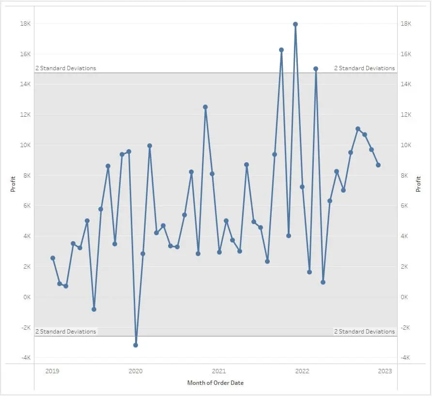
The Z-Score method works by identifying time points in a time series that deviate significantly from the estimated mean and standard deviation over a historical period. This method is a statistical technique used across various fields like finance, meteorology, and healthcare. The formula for the Z-Score is
\[Z = { X - \mu \over \sigma}\]where X is the data point, $\mu$ the mean, and $\sigma$ the standard deviation.
Drawbacks and Mitigation
While simple and widely applicable, the Z-Score method can be overly sensitive to extreme values, especially in datasets with non-Gaussian distributions. Since time series data often violates the assumption of normality, the estimates can be sensitive to anomalies themselves. Using robust statistical estimators like median, interquartile range especially in skewed distributions is advised, which provides more reliable measures of central tendency and dispersion for temporal data. A benefit of the simplified thresholding approach is that Z-Scores are computationally inexpensive to apply even on high frequency streaming data.
Real-World Scenario:
In stock market analysis, Z-Score can identify stocks with unusual price movements. For instance, a stock with a Z-Score beyond +3 or -3 could indicate significant deviation from typical market behavior, prompting further investigation into causes like market news or company-specific events.
Code Implementation
import pandas as pd
data = pd.Series([...])
outliers = data[abs(data - data.mean()) > 2 * data.std()]
2. Moving Average Analysis: Simple Moving Average (SMA)
Application and Theory
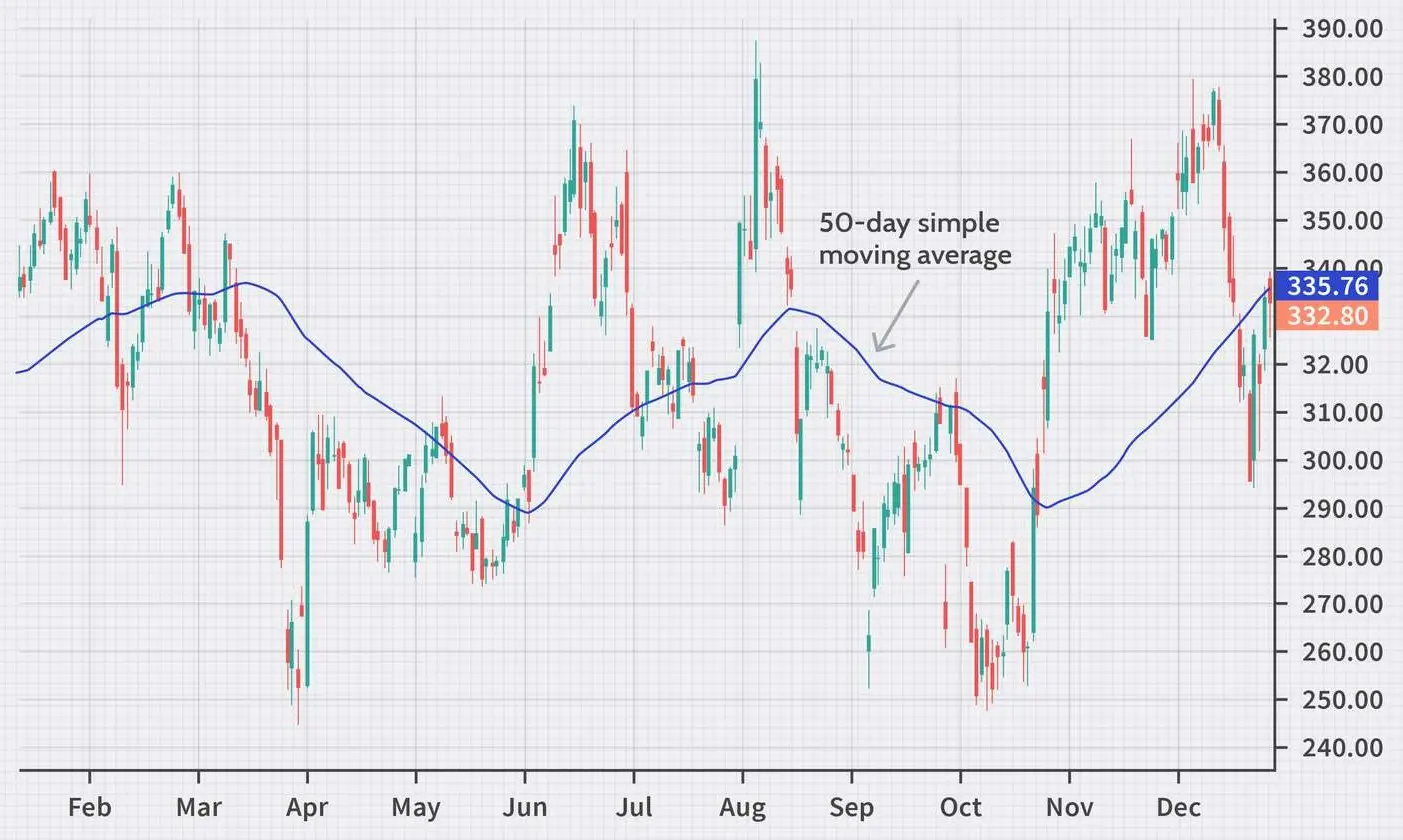
Simple moving averages provide a straightforward way to smooth short-term fluctuations in time series and uncover longer-term trends. By taking unweighted averages across rolling windows of data points over time, SMAs can indicate deviations from the recent local trend.
SMA is frequently used in time-series data analysis, especially in stock trading and meteorological data. It smoothens the time-series data by averaging data points over a specific window. The formula is
\[SMA = { {\sum_{i=1}^N X_i }\over N }\]where N is the window size.
Drawbacks and Mitigation
A key limitation of the Simple Moving Average (SMA) is its lagging performance in volatile datasets, as it fails to swiftly detect abrupt anomalies. By equally weighting all data points in the window, SMAs display reduced sensitivity to current irregularities compared to Exponential Moving Averages (EMAs). While expanding SMA timeframes can dynamically track baseline shifts, accuracy deteriorates over extensive periods as outdated information persists.
To counteract this lag, EMAs emphasize the most recent values via exponential weighting factors. This weighting scheme enables quicker responses to emerging development in the time series data.
Real-World Scenario: Meteorology Meteorologists use SMA to track temperature trends. An unusually hot day in a temperate climate, significantly deviating from a 30-day SMA, could signal an extreme weather event, prompting alerts and further climatic analysis.
Code Implementation
rolling_mean = data.rolling(window=7).mean()
deviation = abs(data - rolling_mean)
outliers = data[deviation > 2 * data.std()]
3. Machine Learning Methods: Isolation Forest
Application and Theory
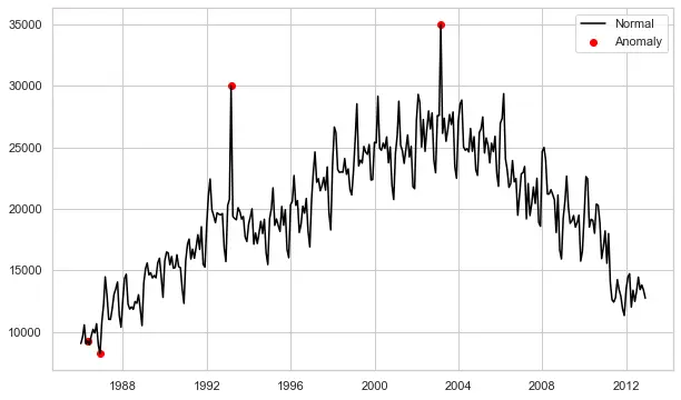
Isolation Forest is an innovative machine learning method extensively used in anomaly detection, notably in fraud detection and network security. Unlike many other techniques, it isolates anomalies instead of modeling the normal points. This algorithm isolates anomalous time points by directly partitioning the data stream using an ensemble of random isolation trees. Since anomalies are few and distinct, they get segregated in just a few partitions compared to normal points.
Drawbacks and Mitigation
A significant limitation of Isolation Forest is its struggle with high-dimensional data, and parameter tuning can be complex. Dimensionality reduction techniques like PCA (Principal Component Analysis) can be employed to address high dimensionality. Careful cross-validation can help in fine-tuning the parameters.
Real-World Scenario: Banking and Fraud Detection
In banking, Isolation Forest is adept at identifying unusual transaction patterns. For example, a series of high-value transactions in a short period, which deviate from a customer’s usual transaction behavior, can be flagged for further investigation as potential fraud.
Code Implementation
from sklearn.ensemble import IsolationForest
model = IsolationForest(n_estimators=100)
model.fit(data.reshape(-1, 1))
scores = model.decision_function(data.reshape(-1, 1))
outliers = data[scores < -0.2]
4. STL Decomposition and LOESS
Application and Theory
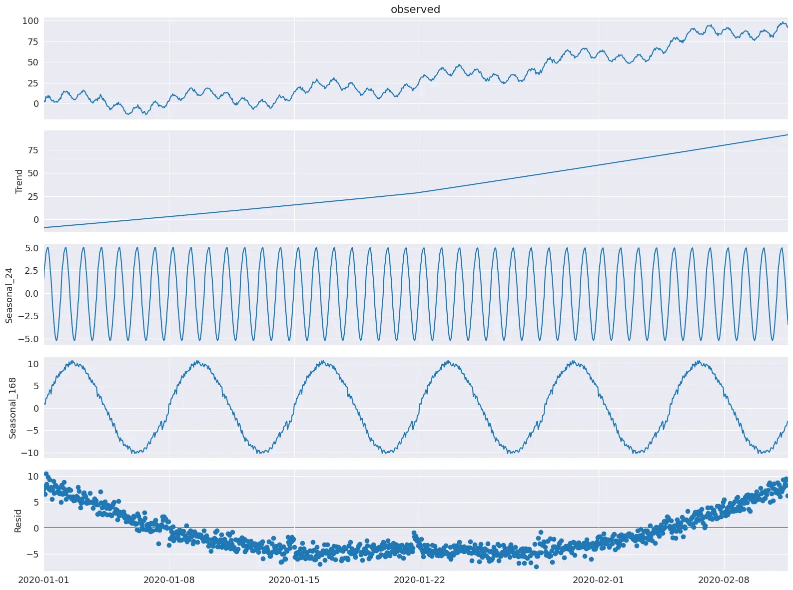
STL (Seasonal and Trend decomposition using Loess) is a robust method used in analyzing time-series data with strong seasonal components, such as economic data or environmental measurements. STL decomposition relies on LOESS locally weighted smoothing to extract seasonal, trend and residual components from a time series while modeling residuals. Anomalies are often found in the residual component, which represents the part of the data that cannot be explained by seasonal and trend components.
Drawbacks and Mitigation
STL may not handle abrupt, non-seasonal changes effectively. To address this, combining STL with other anomaly detection methods, like statistical thresholding on the residuals, can improve its sensitivity to abrupt changes.
Real-World Scenario: Environmental Data Analysis
In environmental monitoring, STL can help in identifying unusual changes in air quality or temperature, which are not part of regular seasonal patterns. For example, a sudden spike in air pollutants in a city could be an indicator of an industrial accident or a significant change in environmental policy.
import statsmodels.api as sm

# Perform seasonal decomposition
decomposition = sm.tsa.seasonal_decompose(data, model='additive')

# Plot the decomposition
decomposition.plot()
As for the threshold function you can use z-score method defined above.
5. Seasonal ESD (S-ESD)
Application and Theory
The algorithm uses the Extreme Studentized Deviate test to calculate the anomalies. In fact, the novelty doesn’t come in the fact that ESD is used, but rather on what it is tested.
The problem with the ESD test on its own is that it assumes a normal data distribution, while real world data can have a multimodal distribution. To circumvent this, STL decomposition is used. Any time series can be decomposed with STL decomposition into a seasonal, trend, and residual component. The key is that the residual has a unimodal distribution that ESD can test.
However, there is still the problem that extreme, spurious anomalies can corrupt the residual component. To fix it, the paper proposes to use the median to represent the “stable” trend, instead of the trend found by means of STL decomposition.
Finally, for data sets that have a high percentage of anomalies, the research papers proposes to use the median and Median Absolute Deviate (MAD) instead of the mean and standard deviation to compute the zscore. Using MAD enables a more consistent measure of central tendency of a time series with a high percentage of anomalies.
Drawbacks and Mitigation
The complexity of understanding and implementing S-ESD can be challenging. Familiarity with the data’s seasonal patterns is crucial. Pre-processing steps like detrending or deseasonalizing the data can help simplify the analysis and improve the method’s effectiveness.
Real-World Scenario: Retail Sales Analysis
In retail, S-ESD can detect unusual sales patterns. For instance, an unexpected spike in sales on a non-holiday weekday might indicate a successful marketing campaign or a data entry error, warranting further investigation.
Resourses: Python module Research paper
Code Implementation
import numpy as np
# Install the below package
import sesd
ts = np.random.random(100)
# Introduce artificial anomalies
ts[14] = 9
ts[83] = 10
outliers_indices = sesd.seasonal_esd(ts, hybrid=True, max_anomalies=2)
for idx in outliers_indices:
    print(f'Anomaly index: {idx}, anomaly value: {ts[idx]}')

6. LSTM-based Autoencoder
Application and Theory
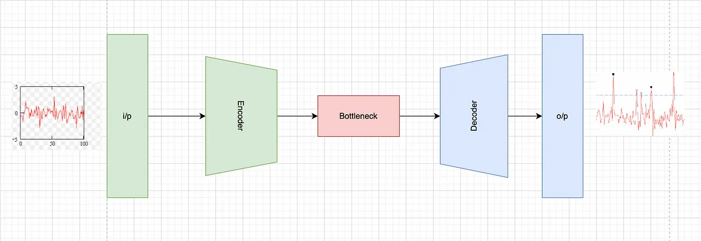
LSTM-based Autoencoders are a deep learning approach, widely used in complex time-series data like IoT sensor data and patient monitoring systems. They employ Long Short-Term Memory (LSTM) networks, a type of recurrent neural network, to learn the normal pattern of the time-series data. Anomalies are detected based on the reconstruction error — the difference between the input and the output of the autoencoder which is often large.
Drawbacks and Mitigation
These models require substantial data for training and significant computational resources. To address these challenges, one can use transfer learning, where a model is pre-trained on a large dataset and fine-tuned with specific data. Additionally, cloud-based computing resources can be leveraged to manage computational demands.
Real-World Scenario: Health Monitoring
In healthcare, LSTM Autoencoders can monitor patients’ vital signs. Anomalies in heart rate or blood pressure readings, differing significantly from the patient’s usual patterns, could indicate urgent medical conditions requiring immediate attention.
Code Implementation
import tensorflow as tf
from tensorflow.keras.models import Sequential
from tensorflow.keras.layers import LSTM, RepeatVector, TimeDistributed, Dense

def create_autoencoder_model(input_shape, encoder_units, decoder_units):
    """Build LSTM Autoencoder model."""
    model = Sequential([
        LSTM(encoder_units, activation='relu', return_sequences=True, input_shape=input_shape),
        LSTM(decoder_units, activation='relu'),
        RepeatVector(input_shape[0]),
        LSTM(decoder_units, activation='relu', return_sequences=True),
        LSTM(encoder_units, activation='relu', return_sequences=True),
        TimeDistributed(Dense(input_shape[1]))
    ])

    model.compile(optimizer='adam', loss='mse')
    return model
After that train the model and make predictions on test data then define your own error and threshold function to flag any anamolies, for example i have created a function to use MSE.
def calculate_error(test_data, predictions):
    """Calculate mean squared error between test data and predictions."""
    print("test_data shape", test_data.shape)
    print("predictions shape", predictions.shape)
    mse = np.mean(np.power(test_data - predictions, 2), axis=1)
    return mse
As for the threshold function you can use z-score method defined above.
7. Wavelet-based Anomaly Detection
Application and Theory
Wavelet-based methods are particularly useful in signal processing and financial time-series analysis. They involve decomposing the time-series data into wavelets which are small waves that can capture both frequency and location in time. This method is adept at identifying anomalies at various frequency levels, which is crucial in signal processing and financial data.
Drawbacks and Mitigation
The primary challenge with wavelet-based methods is their complexity and the expertise required in signal processing. A possible mitigation strategy is to use automated wavelet selection tools and libraries that simplify the process of wavelet transformation.
Real-World Scenario: Stock Market Analysis
In finance, wavelet-based anomaly detection can be used to spot unusual stock market activity. For instance, irregularities in the high-frequency components of stock price movements might indicate algorithmic trading anomalies or market manipulation.
Code Implementation
import pywt
wavelet_coefficients = pywt.wavedec(data, 'haar')
As for the threshold function you can use z-score method defined above.
8. ARIMA-based Outlier Detection
Application and Theory
ARIMA (AutoRegressive Integrated Moving Average) models are a staple in the field of time-series analysis, especially in economic and financial forecasting. They are designed to describe autocorrelations in time-series data. ARIMA models the data as a linear function of its past values (autoregressive part), the past error terms (moving average part), and integrates the need to difference data in case of non-stationarity.
Drawbacks and Mitigation
The primary challenge with ARIMA is its reliance on data being stationary and the complexity in selecting the right model parameters (p, d, q). Augmented Dickey-Fuller tests can be used to check for stationarity, and tools like auto_arima in Python can automate the process of parameter selection.
Real-World Scenario: Economic Forecasting
In economics, ARIMA can be used to forecast key indicators like GDP growth or unemployment rates. Anomalies in these forecasts, such as unexpected drops or spikes, could indicate significant economic events, prompting policymakers and analysts to investigate further.
Code Implementation
from statsmodels.tsa.arima_model import ARIMA

arima_model = ARIMA(data, order=(p, d, q))
model_fit = arima_model.fit(disp=0)
residuals = model_fit.resid

9. Deep Learning: Convolutional Neural Networks (CNN)
Application and Theory
Convolutional Neural Networks (CNNs), commonly associated with image processing, are increasingly being applied to time-series data for complex pattern recognition tasks. CNNs can process time-series data by treating it similarly to an image, extracting features through convolutional layers, and identifying unusual patterns. This data driven feature extraction combined with classification contrasts reconstruction error based approaches till now we have discussed.
Drawbacks and Mitigation
CNNs require large datasets for training and significant computational resources. Using pre-trained models and employing techniques like data augmentation can help in scenarios with limited data. Cloud computing platforms can provide the necessary computational power. And also we should monitor for concept drift to keep model performance from deteriorating.
Real-World Scenario: Biometric Security Systems
In security systems, CNNs can analyze biometric data patterns, such as fingerprints or facial recognition data. Anomalies detected by CNNs might indicate fraudulent attempts at access, prompting security alerts.
Code Implementation
from keras.models import Sequential
from keras.layers import Conv1D, MaxPooling1D, Flatten, Dense

model = Sequential()
model.add(Conv1D(filters=64, kernel_size=2, activation='relu', input_shape=(n_steps, n_features)))
model.add(MaxPooling1D(pool_size=2))
model.add(Flatten())
model.add(Dense(50, activation='relu'))
model.add(Dense(1))

model.compile(optimizer='adam', loss='mse')
Resourses: Research paper
10. Change Point Detection
Application and Theory
Change point detection is used to identify points in time where the statistical properties of a time-series change significantly. This method is crucial in domains like climate monitoring, where it’s important to detect shifts in environmental conditions, and in quality control, to identify shifts in manufacturing processes.
Drawbacks and Mitigation
One challenge with change point detection is distinguishing between actual change points and random fluctuations. Combining this method with other statistical tests or using Bayesian approaches can improve accuracy in distinguishing true change points from noise.
Real-World Scenario: Climate Monitoring In climate data analysis, change point detection can identify shifts in temperature trends, signaling potential climate change events. Detecting these change points can be crucial for initiating environmental policy changes.
There are numeerous algorithms using which we can perform this analysis, below shown is using Bayesian changepoint algorithm.
Resourses: Python Module Python Module
11. Robust Random Cut Forest (RRCF)
Application and Theory
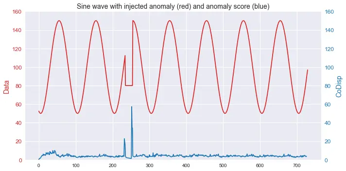
The Robust Random Cut Forest (RRCF) algorithm is a relatively new method, particularly effective for real-time anomaly detection in streaming data, such as financial transactions or IoT sensor data. It constructs a collection of decision trees, called a ‘forest’, to isolate outliers. The isolation is based on the principle that random partitions in the data will isolate anomalies more quickly than normal points.
Drawbacks and Mitigation
RRCF can be computationally intensive for very large datasets. To mitigate this, one can use a subset of the data for training or employ distributed computing frameworks for large-scale data processing. Moreover this Works better than isolation forests with drifted data.
Real-World Scenario: IoT Monitoring
In IoT, RRCF can be used to monitor sensor data for anomalies, such as detecting unusual patterns in temperature or pressure readings in an industrial setting, which might indicate equipment malfunctions or environmental hazards.
Resourses: Python Module
import numpy as np
import rrcf

# Generate data
n = 730
A = 50
center = 100
phi = 30
T = 2*np.pi/100
t = np.arange(n)
sin = A*np.sin(T*t-phi*T) + center
sin[235:255] = 80

# Set tree parameters
num_trees = 40
shingle_size = 4
tree_size = 256

# Create a forest of empty trees
forest = []
for _ in range(num_trees):
    tree = rrcf.RCTree()
    forest.append(tree)

# Use the "shingle" generator to create rolling window
points = rrcf.shingle(sin, size=shingle_size)

# Create a dict to store anomaly score of each point
avg_codisp = {}

# For each shingle...
for index, point in enumerate(points):
    # For each tree in the forest...
    for tree in forest:
        # If tree is above permitted size...
        if len(tree.leaves) > tree_size:
            # Drop the oldest point (FIFO)
            tree.forget_point(index - tree_size)
        # Insert the new point into the tree
        tree.insert_point(point, index=index)
        # Compute codisp on the new point...
        new_codisp = tree.codisp(index)
        # And take the average over all trees
        if not index in avg_codisp:
            avg_codisp[index] = 0
        avg_codisp[index] += new_codisp / num_trees
12. Bayesian Structural Time Series (BSTS)
Application and Theory
Bayesian Structural Time Series (BSTS) is a probabilistic approach, used extensively in econometrics and marketing analytics. It models time-series data as a combination of components like trend, seasonality, and holidays, using Bayesian methods to estimate these components’ contribution and detect anomalies. Anomalies reflected as noise in seasonally adjusted series.
Drawbacks and Mitigation
BSTS can be complex to understand and implement, particularly in choosing priors. Using software packages that provide default settings for priors can simplify its application.
Real-World Scenario: Marketing Analytics In marketing, BSTS can analyze sales data to understand the impact of marketing campaigns. An unexpected dip or rise in sales, when controlled for seasonal and holiday effects, might indicate the success or failure of a campaign.
Resourses: Python Module Python Module