Made by
- Sai Vinay Teja Jakku - jakku.s@northeastern.edu
- Akarsh Singh - singh.akar@northeastern.edu
- Janvi Shetty - shetty.j@northeastern.edu
- Anurag Palanki - palanki.a@northeastern.edu
Problem Setting & Definition:
Over the past few years, business owners and retailers, big or small, have started taking their shops online to increase their reach, promote their brand and increase sales that cover a wide range of customers. For these businesses, it is essential to identify the customer base and give them enough rewards and incentives to encourage their online purchase. The primary objective of this project is to identify patterns of the customers that browse a website and make a successful purchase. We intend to achieve this by using various Machine learning techniques and selecting the best classification algorithms that successfully classify the revenue promoting customers from other users using the Online Shoppers’ Purchasing Intention dataset.
Data Sources:
Data Description:
Of the 12,330 sessions in the dataset, 84.5% (10,422) were negative class samples that did not end with shopping, and the rest (1908) were positive class samples ending with shopping[1]. The dataset was created so that each session would belong to a different user in a year to avoid any tendency to a specific campaign, special day, user profile, or period. It contains ten numerical and seven categorical columns, with the 8th and target column being the target column.
Splitting The Dataset:
Before we started training, the first step we took was to split the data into train and test data sets. We trained the model using the training dataset and evaluated the fit model using the test dataset. We also have split the data into folds for k-fold cross-validation for one of the machine learning models. Splitting the dataset into train, validation and test data helps in removing bias and in hyper-tuning the parameters.
Exploratory Data Analysis and Visualization:
To get a complete overview of the dataset we were dealing with, we created a function that described the dimensions. The description includes the categorical attributes, numerical attributes, number of null values in all the columns and many more.
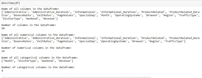
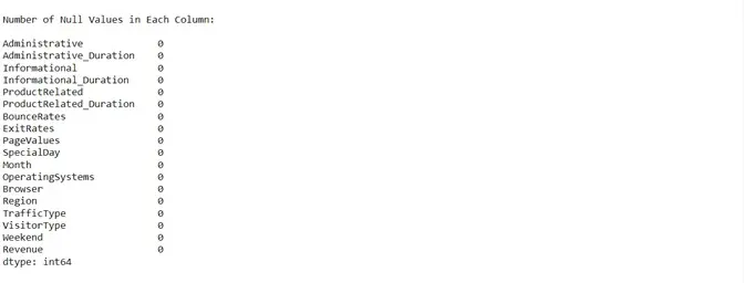
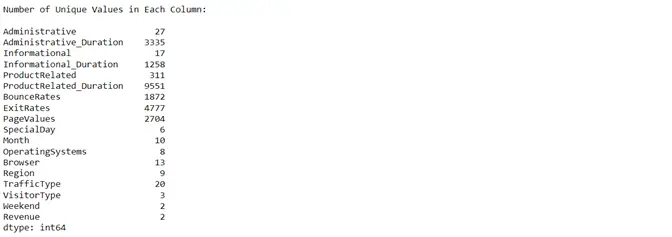
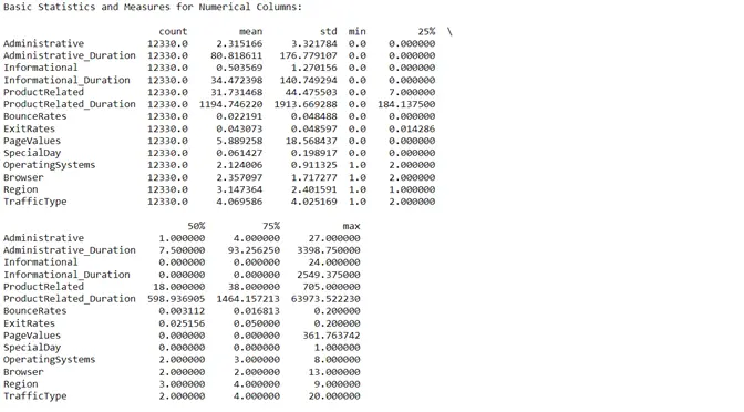
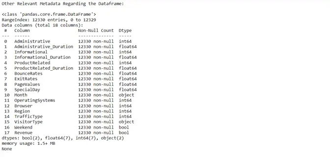
All the attributes of the dataset contained non-null values. Hence, null value processing was not required. We then shifted our focus towards finding the correlation of each attribute with every other attribute in the table to remove recursive information.
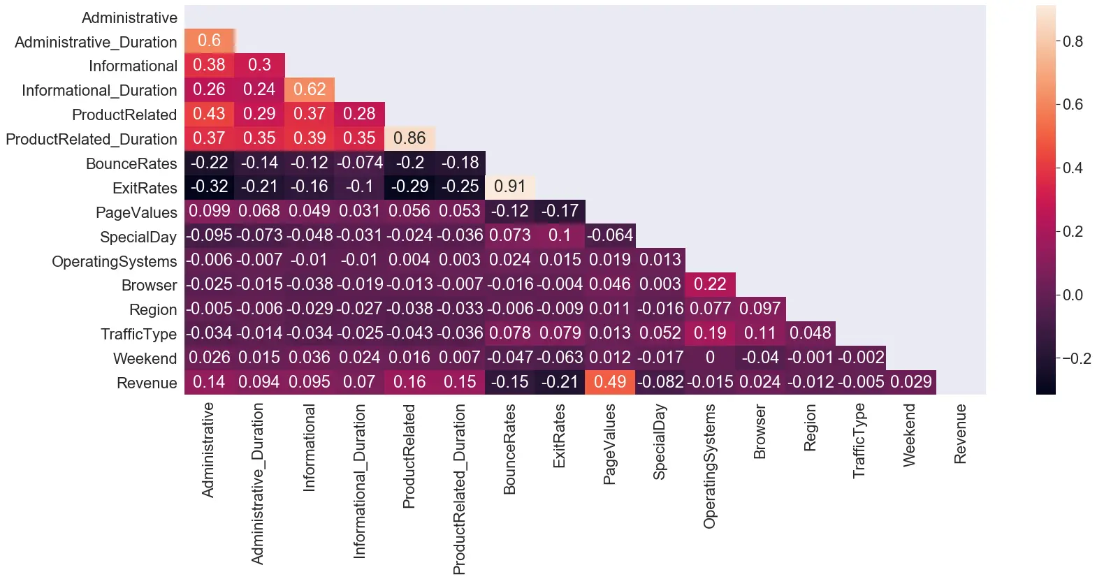
We see a high correlation between the ‘BounceRate’ and the ‘ExitRates’ (0.91) and between the ‘ProductRelated_Duration’ and the ‘ProductRelated’ (0.86). These columns were dealt with while Feature selection.
We plotted a bar plot to find the count values of the two classes in our dataset.
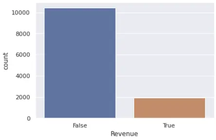
The number of false cases heavily outweighs the number of True classes. From this graph, we realised that we had to work with the skewness in data by either upsampling or down-sampling the data while passing the training data sets into the model.
To evaluate the distribution of values of the columns with relatively high correlation values with the ‘Revenue’ column, a bar plot was used.
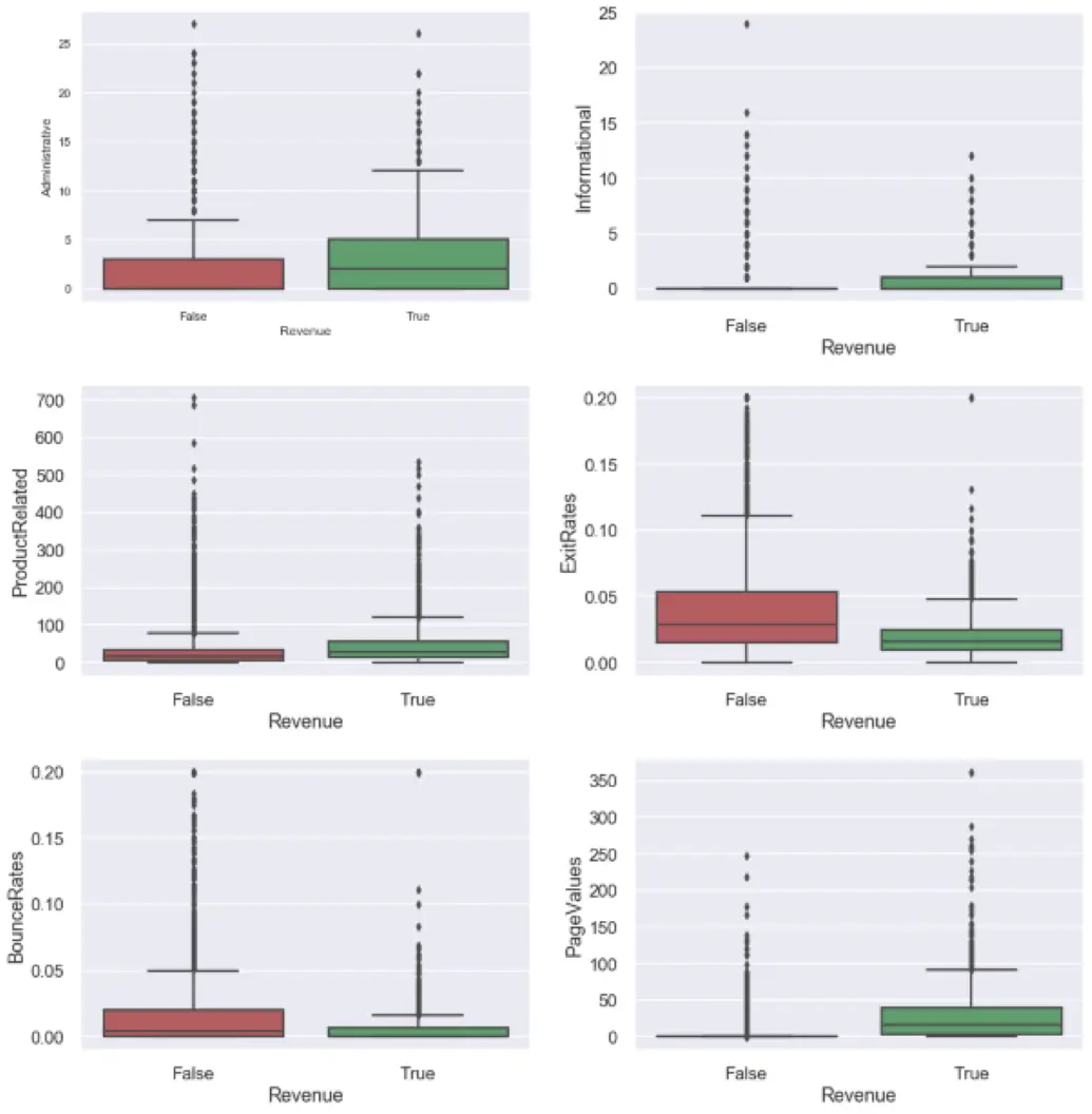
The data is highly skewed concerning revenue with many outliers. The skewness of the columns is dealt with while the skew handling process and the outlier and dealt with during Data preprocessing and cleaning.
In the next part, we checked for the linear separability of the two classes for the subset of the total number of attributes in our dataset. We used a grid plot for this case. The lower diagonal shows the kernel density estimate of the distribution concerning the attribute pairs, the upper diagonal shows the scatter plot of the same attribute pairs and the diagonal shows the distribution of attribute values across the dataset using kernel density estimate plot. The ‘TotalDuration’ here denotes the summation of the ‘Administrative_Duration’, the ‘Informational_Duration, and the ‘ProductRelated_Duration’.
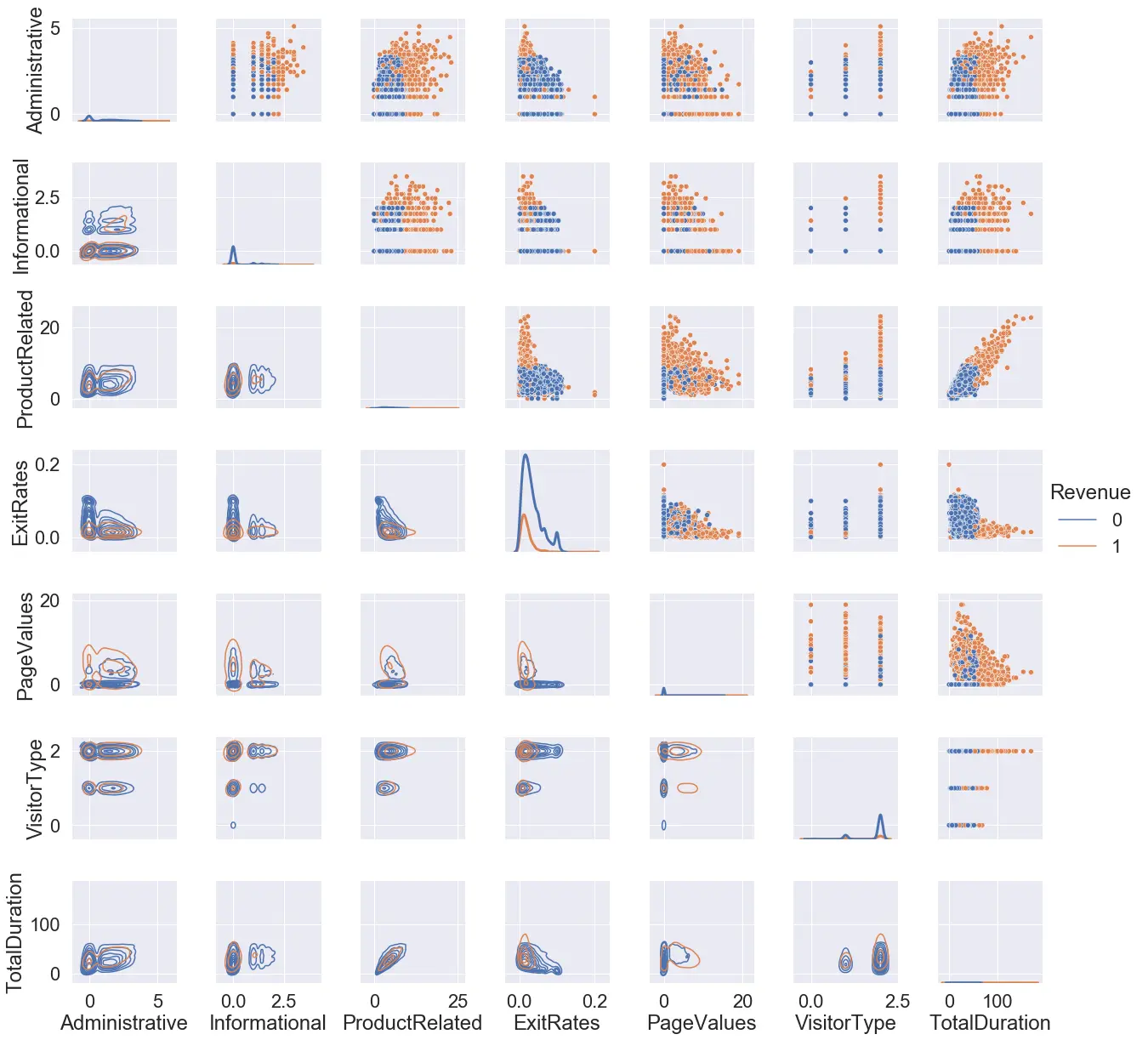
From the data, we can see that the concentration of the 2 classes and mostly overlapping in all the cases. To the best of our knowledge, we see no separability of these classes when represented in 2-dimensional space.
Feature Selection:
On the basic of descriptive statistical analysis of the dataset concerning the target class (Revenue), a few problematic instances have to be addressed, that are intrinsic to the dataset. First, there is a major class imbalance, approximately 1:5 to the class of interest. This calls for data transformation and stringent feature selection to create a generalised model capable of correctly identifying the minority class. (i.e. the class of interest) Second, almost all the non-categorical variables are significantly skewed to the right and possess significant outliers. Unless taken care of, the model will have significant bias, would not be able to generalise well, and would be susceptible to missing out on tricky instances of minority class data points. Third, on performing correlation analysis all features present are either weakly correlated or uncorrelated to the target class, except one. If features are not created or data processing is not performed to somehow increase correlation bias would increase for model training and performance will be compromised. A good thing about the dataset is that there are not any null values hence, dealing with null values before processing is altogether eliminated.
The following steps were taken after multiple iterations of trial, and testing, and based on positive statistical impact concerning change:
- All numerical variables with a Pearson correlation coefficient in the range [-0.1,0.1] for target variable (y) were dropped as their impact on prediction would be insignificant.
- Attributes like administrative and administrative duration were highly correlated, this led to a multi-collinearity issue that is undesirable for model training. Hence, one variable from three pair of similar variables were dropped.
- We created a new feature by performing a weighted sum of all the duration variables and called it ‘total_duration’. These 3 variables were then dropped as addressed in the previous point.
- We created a new feature by performing a weighted sum of all the duration variables and called it ‘total_duration’. These 3 variables were then dropped as addressed in the previous point.
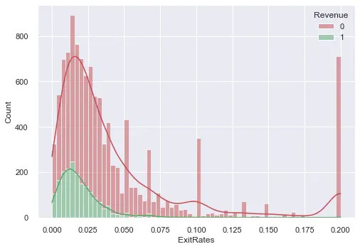
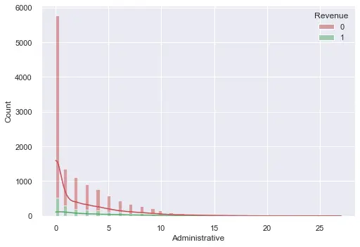
- This process was followed by outlier detection and removal. We visualised each variable to the target class as a stacked histogram with a KDE plot before removing unwanted data points. We noticed that almost all variables are right-skewed and mostly because of the majority class. Due to the nature of our imbalanced dataset, we only removed outliers from target label 0 to reduce skewness and improve the imbalance ratio. The method used for removing outliers was that of quartiles. The steps are shown below.
- Find q25th, q50th, and q75th quartile along with interquartile range (IQR, i.e. q75th – q25th quartile)
- A constant k (1.5 -2.5) is chosen as a multiplicative factor to be multiplied by IQR to determine scrutiny of outliers. This is subjective to the situation and data. Let’s call (k)x(IQR) as s
- We then classify values to the left of q25th – s and that to the right of q75th + s as outliers and remove them
- Since our dataset is skewed to the right, there were no outliers whatsoever beyond q25th – s, when then removed all outliers belonging to class 0 of the target label (y)
A couple of examples are shown below for outlier detection:
- Lastly the data frame was normalised to a standard scale before feeding it into a model.
Post outlier treatment 17.28% of the dataset size was reduced where 2131 data points from majority class 0 were dropped. The final correlation map looked as follows (Revenue being the target class)

Upscaling:
Since the target class is a minority class, we have decided to upscale the target class using the Synthetic Minority Oversampling Technique also known as SMOTE to balance the dataset. It is done before fitting the data to the model and does not give any additional information to the model.
SMOTE first selects a minority class instance ‘a’ at random and finds its k nearest minority class neighbours. The synthetic instance is then created by choosing one of the k nearest neighbours ‘b’ at random and connecting a and b to form a line segment in the feature space. The synthetic instances are generated as a CONVEX combination of the two chosen instances-a and b. This data augmentation technique is effective because it creates samples that are relatively close in feature space to existing examples from the minority class.
Model Implementation:
Following are the different Machine Learning Models we Implemented For Classification:
- Logistic Regression
- Gaussian Naive Bayes
- Neural Network
1. Logistic Regression:
It is a form of statistical software that analyses the association between a dependent variable and one or more independent variables by estimating probabilities using a logistic regression equation.

This analysis can help anticipate the likelihood of an event or a choice occurring. The output obtained in the case of logistic regression is always between (0 and 1), which is suitable for a binary classification task. The higher the value, the higher the probability that the current sample is classified as class= 1, and vice versa. It takes both continuous and discrete variables as input. The data fed into the model is upscaled on the minority class.
Cross Validation:
Cross-validation is a resampling method that uses different data portions to test and train a model on each iteration. It is a robust measure to prevent overfitting. The complete dataset is split into parts. In standard K-fold cross-validation, we need to partition the data into k folds. Then, we iteratively train the algorithm on k-1 folds while using the remaining holdout fold as the test set. In our case, we chose the k to be 5.
Algorithm:
- The dataset values are split into training and testing sets. The training set is up-scaled using the smote function to take into account the biassed number of true to false values in the target variable.
- The training data is split into 5-subsets on which 5-fold validation is performed. An array is created to store the gradient calculated for each cross-validation.
- In every fold, we initialize the gradient term to zero and pass it to a function that calculates the optimal gradient term taking into account the maximum number of iterations.
- A threshold is set while calculating the change in the gradient taking into account the set tolerance value by the user to prevent overfitting.
- The set value is added to the array initially defined for storing the optimal gradient in each fold.
- The gradient values are then averaged to the number of folds taken for cross-validation, and this gradient term is used for the evaluation of the validation data.
Logistic Regression Results:
We tried tuning the parameters such as learning rate and tolerance here are a few of them
| Tolerance | Learning Rate | Accuracy | F1 | Recall | Precision |
|---|---|---|---|---|---|
| 0.00001 | 0.001 | 0.9023 | 0.7060 | 0.6749 | 0.7401 |
| 0.001 | 0.01 | 0.9051 | 0.7352 | 0.7584 | 0.7133 |
| 0.01 | 0.1 | 0.8968 | 0.7362 | 0.8284 | 0.6624 |
| 0.0001 | 0.0001 | 0.8956 | 0.6453 | 0.5463 | 0.7883 |
The balanced results are given with a learning rate of 0.1 and tolerance of 0.01 concerning the target class i.e Revenue.
The best results were given with a learning rate of 0.1 and a tolerance of 0.01. The test accuracy obtained was 0.89, with precision and recall as 0.66 and 0.82. This is a much better balance when compared to our baseline logistic regression model (threshold 0.5) which had a precision and recall of 0.78 and 0.47 respectively whereas our model gave the best results with a threshold value of 0.9.
2. Gaussian Naive Bayes
Gaussian Naive Bayes assumes that each class follows a Gaussian distribution. As our dataset contained two classes (True and False), the Dataset did not have to go through any manipulation to be fed into the code. Priors were simple. We parsed the target value of the training set which was upscaled before the calculation to find the average number of true and false values in it.
We already assumed that the distribution of values in the columns is gaussian, so for each dimension, mean and standard deviations are calculated. For any new point, we look into the probability distribution of the dimension values to find the probability of it belonging to the respective distribution. The function used is:

Algorithm:
- The dataset values are split into training and testing sets. The training set is up-scaled using the smote function to take into account the biassed number of true to false values in the target variable.
- The training data is split data comprising the two classes, which are to be classified.
- The priors and distribution for respective classes are calculated using the sub-datasets that were taken in the previous step.
- Once the probability values are calculated for each class, the calculated values are then used for the prediction of the test set.
Gaussian Naive Bayes Results:
Metrics for result comparison used are the Accuracy, Precision, Recall and the F1 score:

The Gaussian Naive Bayes gave poor performance values compared to our baseline model (which is our Logistic regression model with a 0.5 threshold). It had a test accuracy and precision of 0.17 and 0.18 respectively and a low F1-Score of 0.3 concerning target class 1. Our baseline model had precision and recall of 0.78 and 0.47 respectively. These stats were expected considering the imbalance in the test data.
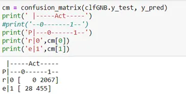
The model recall value is high because of the highly skewed classification. As seen above, the model tends to classify the majority of the observations to class 1 which is our target class, which is not a desirable outcome. Thus, from the results seen here, this model should not be considered for our dataset given the highly skewed distribution.
3. Neural Networks
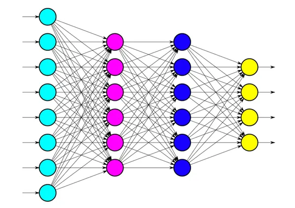
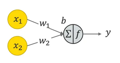
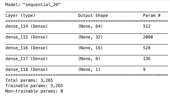
Here, we have used fully connected neural networks with 1 input layer, 2 hidden layers, and a final output layer when the sigmoid function is applied to give a probability between 0 and 1 for the respective classes. This class of networks consists of multiple layers of computational units, usually interconnected in a feed-forward way. Each neuron in one layer has directed connections to the neurons of the subsequent layer. In many applications, the units of these networks apply a sigmoid function as an activation function. Other functions include tan(h), relu, etc. A basic structure of a single node is displayed below:
The model summary for the final model used is as shown below:
Bias-Variance Trade-off:
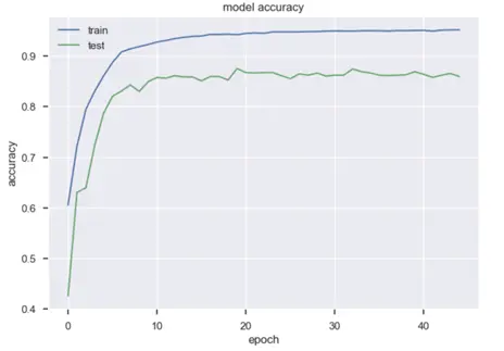
We monitored the validation loss in tandem with the training loss and the number of epochs to see how it changes. Initially starting with a higher number of iterations (epochs) we noticed that the validation loss is increasingly fluctuating from a minimum point, this meant that the model was overfitting. We balanced that off by reducing the number of epochs. After that, we noticed that the validation accuracy was increasing which meant that the model would generalise well.
Neural Networks Results:
The neural network was our best-performing model that generalised well. It had a test accuracy of 0.90. But more importantly, precision and recall of 0.74 and 0.75 respectively concerning the target class 1. This is a much better balance when compared to our baseline logistic regression model (threshold 0.5) which had a precision and recall of 0.78 and 0.47 respectively. These stats are good considering the sheer class imbalance in the test data. In simpler terms, the model is capable of recognizing every 3/4 true labels correctly. Accuracy is high because many 0-class data points can be identified easily.
Some additional results obtained are shown below in the form of a table:
| Epochs | Batch Sizes | Accuracy | F1 | Recall | Precision |
|---|---|---|---|---|---|
| 50 | 256 | 0.8784 | 0.6517 | 0.5930 | 0.7232 |
| 150 | 512 | 0.8925 | 0.7140 | 0.6994 | 0.7292 |
| 150 | 256 | 0.9004 | 0.745 | 0.7587 | 0.7318 |
| 150 | 64 | 0.8941 | 0.7294 | 0.7444 | 0.7151 |
Final Results:
The granularity and nature of the dataset bought challenges that needed to be handled to generate a generalised usable predictive model. Through the processes, most time was spent on understanding nuances of the features from a statistical standpoint and selecting the best ones based on evidence and standard procedures. Upscaling was also important to elevate our class of interest and SMOTE does a good job in the mix for the same. We included multiple classification algorithms and gauged the pros and cons for each. Fully connected neural networks outperform other algorithms for our case by having high precision and recall values that are also close to each other. Logistic regression also gave us good results. We also note that the best results were obtained when the threshold value for positive classification was over 0.8. This shows that due to the sheer amount of class imbalance in the test set, it is better to classify a datapoint as positive until the model is highly certain. As not a part of our course, decision tree-based models were not tested for this project.
Citation:
- Sakar, C. & Kastro, Yomi. (2018). Online Shoppers Purchasing Intention Dataset, UCI Machine Learning Repository
- Page 47, Imbalance Learning: Foundations, Algorithms, and Applications, 2013