Team Details:
- Ayush Soni - soni.ay@northeastern.edu
- Divyangana Pandey - pandey.di@northeastern.edu
- Radhika Jayachandran - jayachandran.r@northeastern.edu
I. Introduction:
Development in industrialization and advancement of technology has led to an increase in pollutant levels in the air. In China, this has led to an increase in extreme weather conditions such as a higher recorded increase in temperature, haze, smog and adverse effects on health conditions to the residents of these areas. The research on the concentration of these pollutants will provide the information required for the improvement of significant health, environmental conditions, and benefits to the economy while reducing costs on solutions to reduce air pollution.
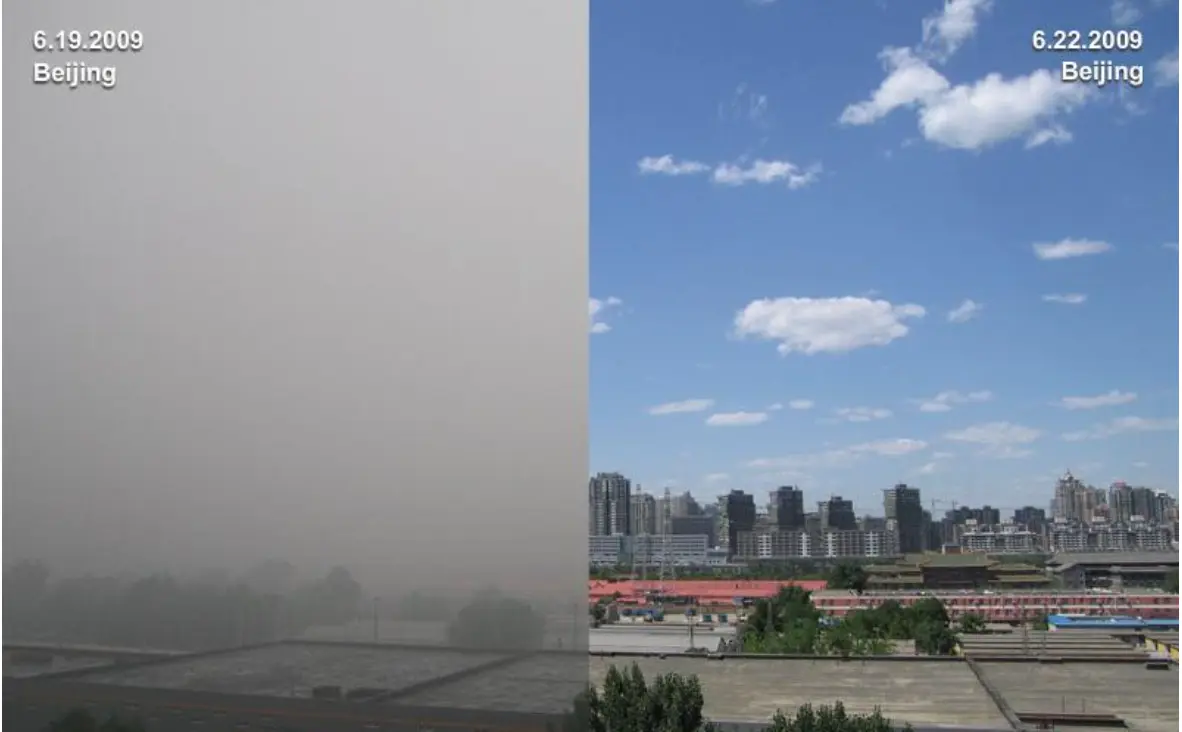
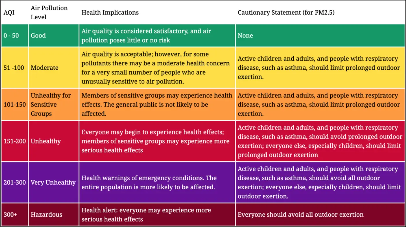
The Air Quality Index is a metric that quantitatively describes the number of pollutants suspended in the air to briefly describe the air quality in an area. The air’s concentration of pollutants such as PM2.5, PM10, CO, O3, SO2 and NO2 indicates the overall air quality. However, other meteorological conditions also play a pivotal role in the quality of air.
I.I. Problem Definition:
Through this project, we aim to research and incorporate complex nonlinear relationships between the concentration of air pollutants and meteorological variables across a given period. Implement and build a prediction system based on individual pollutant concentration levels that can predict air quality. Doing so will make the information on the air quality index more flexible and useful. Systems that can generate warnings based on air quality are required and important for a change as they may play an important role in health alerts when air pollution levels may exceed specified levels. By the end of this classroom project, we aim to establish a relationship between the concentration of pollutants and its correlation with AQI (Air Quality Index).
II. Data Description:
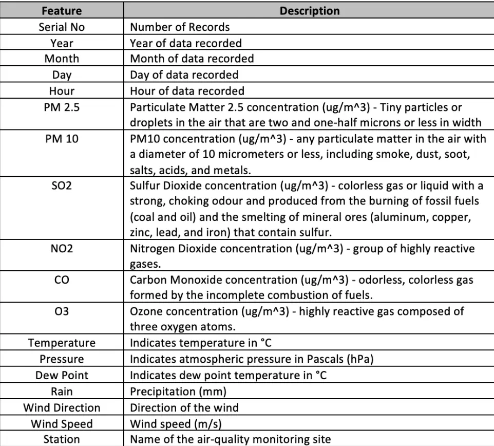
The dataset was procured from the very versatile website for the Data Science dataset, UCI ML. The dataset records hourly pollutant concentrations from twelve different controlled air quality monitoring centres across China.
II.I. Data Features:
The data set selected by us comprises of eighteen dimensions and four lakh instances across the timeline of March 1st, 2013, to February 28th, 2017. Below we listed the types of features to gauge a better understanding of our data:
II.II. Data Cleaning and Preprocessing:
To prepare the data for exploration and model fitting, we first combined the data files that were separated by record for each unique station. After combining these files we performed various exploratory data analyses to study and understand the recorded data and the following were the changes made to attain our target:
- Columns ‘year’, ‘month’, ‘day’ and ‘hour’ were combined to create a Date – Time column such that we can distinguish the records per each day per time.
- There were no duplicate records of Date – Time in the dataset, hence no rows were dropped.
II.III. Feature Engineering
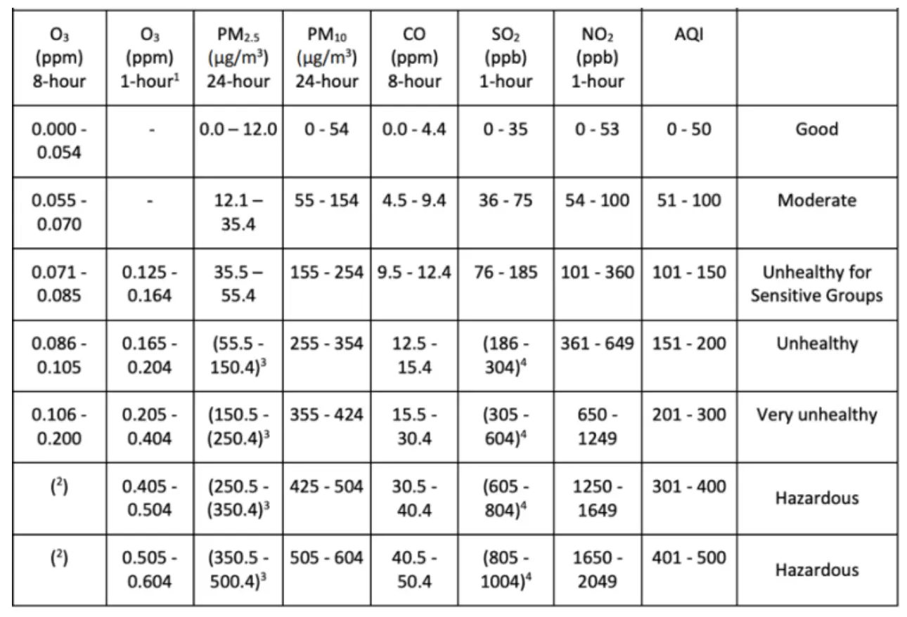
The recorded data for these pollutants were converted to their standard unit from the recorded unit. The above calculations were achieved by the formulae:

- All Null values within the data were replaced by their median for each day recorded by each station. While checking the data we noted that there exist days with a whole 24-hour period where no data was recorded. We replaced these null values with 0.
- Further to obtain the AQI Index of individual pollutants, a rolling window average for each pollutant must be obtained. This data is then segregated into various classifications of AQI and the max value is recorded as the quality index for the given day. The category of AQI is defined as per the standardized government information.
- AQI is calculated using the formula given below:

II.IV. Data Exploration:
Pie Chart - Percentage of Days Within Each Air Quality Classification:
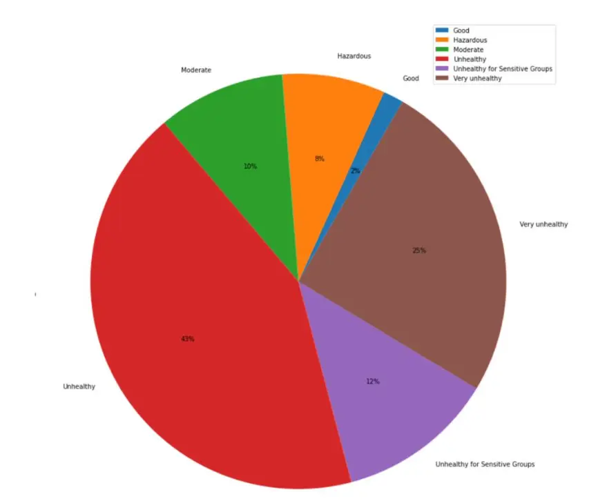
Python has functional visualization libraries that can explore and project your data in creative and pictorial ways. Here we plotted a pie chart of the count of different AQI indexes to show where the air quality stands within the region.
Box Plot – Air Quality Index Across Months:
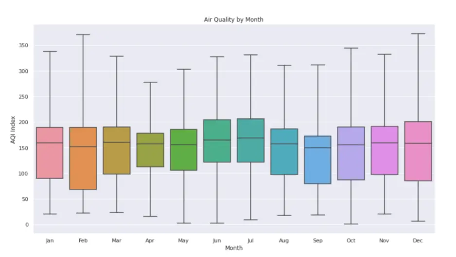
The boxplot gives us a picture of the ranges of AQI for each month to get an idea of which months have the best air quality and the average air quality across each month.
Heat Map – Correlation Matrix Between Input Features:
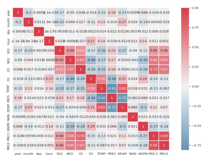
As we can see above the heat map gives us the level of correlation between our input features from the dataset. This can help remove features that are highly correlated.
Time series – Pollutant Concentration Across Time:
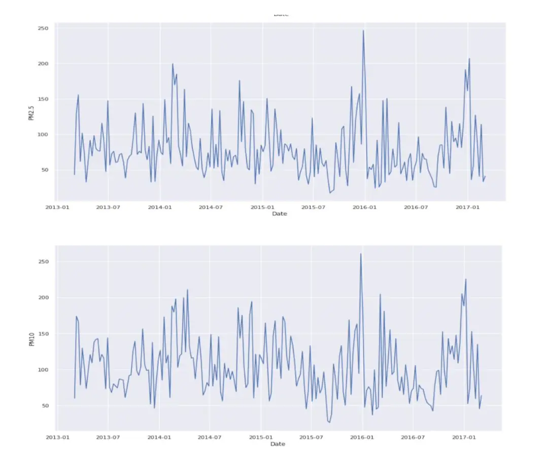
The time series gives us the effect of each pollutant and its curve on air quality over the years.
III. Model Implementation:
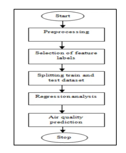
We processed and analyzed our data through regression models to obtain accurate predictions. Machine learning models use techniques that find the relationship between dependent and independent variables. These techniques can be used in forecasting, prediction, time series modelling etc. Some of the modelling techniques we learned in the classroom setting that can be applied accurately in our AQI prediction project are Linear regression, Logistic regression and Naïve Bayes.
III.I. Linear Regression:
Linear regression is a method of fitting independent variables with dependent variables into a line in n dimensions where n is the total number of features or variables within our data. The model also minimizes the total error while trying to fit all the data points in one line and learning continuously by optimizing parameters. Optimization is carried out by using gradient descent. Gradient descent partially derives the loss function and all parameters are updated by subtracting the previous value with the derivative time the learning rate. The learning rate is tuned by the trial and error method. The equation of multivariate linear regression is given by:

Where, Yi = estimate of ith component of dependent variable y n = independent variables
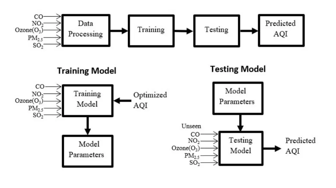
Results:
The linear regression model was run for various parameters in order to obtain the most accurate results.

III.II. Logistic Regression:
The primary idea behind Logistic regression is to establish a relationship between an input feature and a predictor variable which is often a categorical one for classification. There are different types of logistic regression models depending upon the number of classes the data is required to be segregated into:
Binary classification: This involves predicting if the sample falls into class 0 or 1. For example, an email is a spam or ham. The sigmoid function is used to calculate values for logistic regression involving two classes. Sigmoid pushes the input values to fall within the range [0,1].

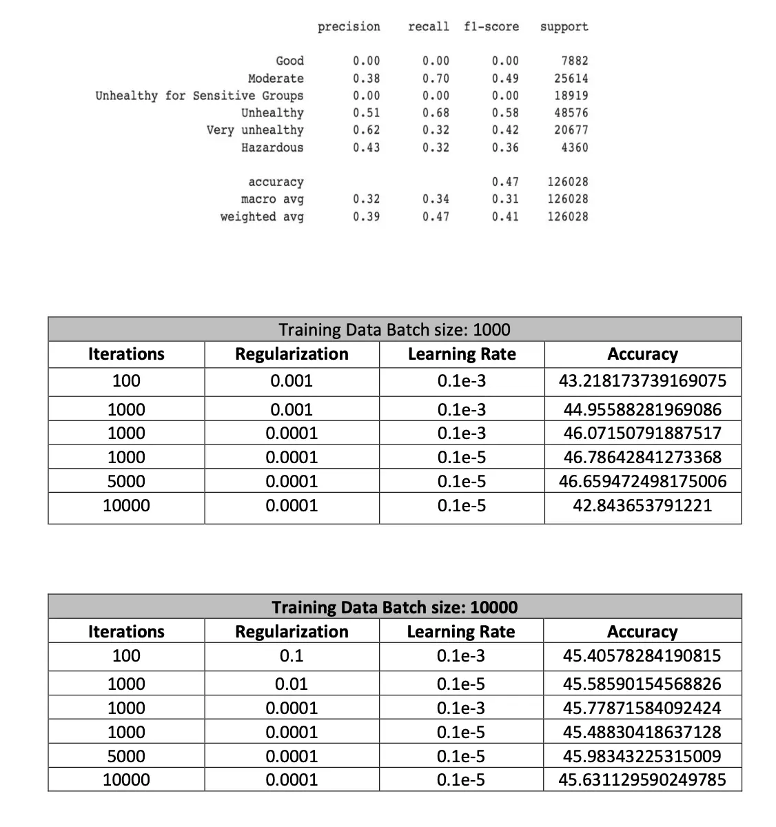
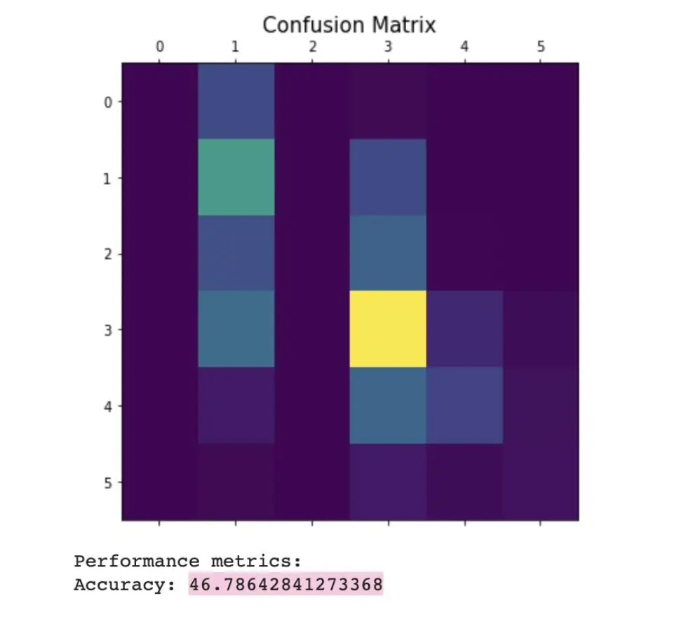
Multiclass logistic regression: It is used to classify records into more than two classes. A SoftMax function is used to calculate the probabilities. For a given sample we calculate the probability of it belonging to each of the n classes. The sum of all probabilities for each sample should add up to 1. We classify a record belonging to a particular class by selecting the one with the highest probability. For our dataset, we have engineered a new column called AQI_encoded by using the below logic. This helps us to fit the data into a multinomial Logistic Regression model. The target classes are one-hot encoded before calculating the probabilities.

Results:
III.III. Naive Bayes:
The core of a Naive Bayes model is prediction, diagnosis and reasoning. Variables generated randomly are represented by nodes and conditional probability is the information between these nodes. We combine conditional probability with prior probability to obtain a posteriori probability in order to achieve the effect of prediction. It is a simple model widely used due to its speed and faster learning rate. Bayes theorem helps us calculate the Probability of A happening provided B has occurred with the assumption of independence.
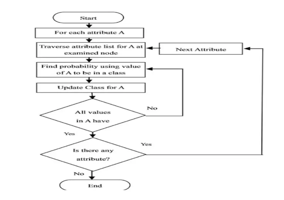
The following formula is used for calculate probability:

The Probability of event Bi occurring such that event A has occurred is given by the above formulae.
The Gaussian Naive Bayes functions are typically derived from probabilities of the lower-order estimates from the training data. These may easily be updated as new training data come in. Because you just need to estimate the mean and standard deviation from your training data, the Gaussian (or Normal) distribution is the simplest to deal with. The assumption that the continuous values associated with each class are distributed according to a normal (or Gaussian) distribution is frequently made when working with continuous data. The characteristics and likelihood is predicated on:

Assuming variance is,
- is independent of Y (i.e., σi),
- or independent of Xi (i.e., σk)
- or both (i.e., σ)
The AQI classification categories were encoded into the below values in order to classify our predictions:

Results:
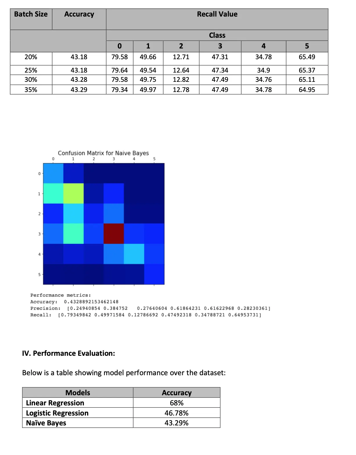
Below are the results obtained by applying batch size to data split while running the model:

V. Conclusion:
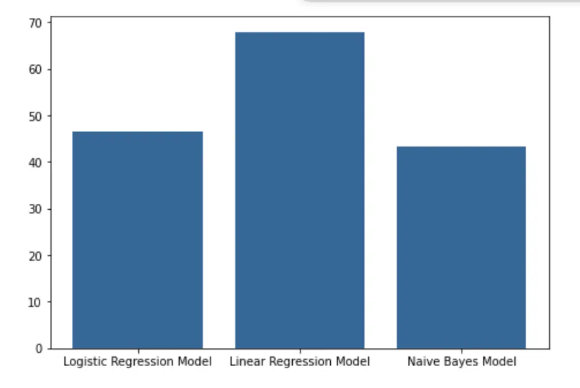
The air quality prediction model based on machine learning is used to predict the air quality in Beijing. The aim of the project was to research and study the various Machine Learning models available in order to implement the best fit for our dataset. As a team, we had the opportunity to clean the data, observe the importance of pollutants and their impact on the quality of air and implement ML algorithms to predict the AQI and observe how the predicted value differs from the original value. The following factors are used for the evaluation of the model, Temp, Pressure, SO2, NO2, O3, CO, PM10 and PM2.5 and the calculated AQI value is used as the target. The model is trained and verified by using the historical data on air quality to obtain comprehensive accuracy. The results show that the Linear Regression model predicted the air quality with a 68% accuracy, followed by Logistic Regression at 46.78% and Naive Bayes at 43.29%. In addition, wind, precipitation and other environmental conditions also play a factor that directly affects the quality of air. Therefore, taking these factors would help further improve the accuracy of our models and is one of the future research directions.
VI. References:
- https://archive.ics.uci.edu/ml/datasets/Beijing+Multi-Site+Air-Quality+Data
- http://www.ijsei.com/papers/ijsei-67117-18.pdf
- https://iopscience.iop.org/article/10.1088/1742-6596/2010/1/012011/pdf
- BC. Liu, et al, “Urban air quality forecasting based on multi-dimensional collaborative Support Vector Regression (SVR): A case study of Beijing-TianjinShijiazhuang”, PLOS, 2017